本节我们将了解神经网络进行非监督形式的学习,即autoencoder自编码
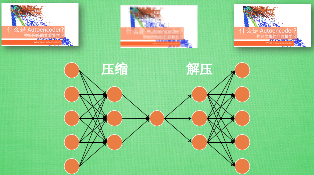
假设图片经过神经网络后再输出的过程,我们看作是图片先被压缩然后解压的过程。那么在压缩的时候,原有的图片质量被缩减,解压时用信息量小却包含所有关键信息的文件恢复出原本的图片。
为什么要这么做呢?
因为当神经网络接收大量信息时,神经网络在成千上万个信息源中学习是一件比较吃力的事。所以进行压缩,从原图片中提取最具代表性的信息,减小输入信息量,再把缩减过后的信息放进神经网络学习,这样学习起来简单轻松许多。
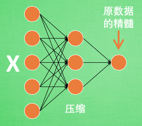
如下图所示,将原数据白色的X压缩,解压还原成黑色的X,求出预测误差,进行反向传递,逐步提升自编码的准确性。训练好的自编码中间一部分就是能够总结原数据的精髓。可以看出,从头到尾,我么值用到看输入数据X,并没有用到X对应的数据标签,所以可以说自编码是一种非监督学习。到了真正使用自编码的时候,通常只会用到自编码的前半部分。

如下图,这部分也叫作encoder编码器,编码器能得到元数据的精髓我们只需要创建一个小的神经网络学习这个精髓的数据,不仅能减少神经网络的负担,同样能达到很好的效果。
至于Decoder解码器,解压器在训练的时候是要将精髓信息解压成原始信息,那么这就提供了一个解压器的作用,甚至我们可以认为是一个生成器。做这件事的一种特殊编码叫做variational autoencoders,其例子就是让它能模仿生成手写数字。

-----------------------------------------------------------------------
自编码 Autoencoder (非监督学习)
我们会首先通过Feature的压缩并解压,将结果与原始数据进行对比,观察处理后的数据是不是如逾期跟原始数据很相像。(这里会用到MNIST数据)
然后我们只看Encoder压缩过程,使用它将一个数据集压缩到只有两个Feature时,将数据放入一个二维坐标系内,特征压缩的效果如下(同样颜色的点,代表分到同一类的数据):

Autoencoder
采用的数据依然是MNIST手写数据集
import tensorflow as tf
import numpy as np
import matplotlib.pyplot as plt

#import mnist data
from tensorflow.examples.tutorials.mnist import input_data
mnist = input_data.read_data_sets("MNIST_data/",one_hot=False)
参数
# Parameter
learning_rate = 0.01
training_epochs = 5 # 五组训练
batch_size = 256
display_step = 1
examples_to_show = 10
MNIST数据,每张图片的大小是28*28pix,即784Features:
# Network Parameters
n_input = 784  # MNIST data input (img shape: 28*28)
- 在压缩环节,我们要把这个feature不断压缩,经过第一个隐藏层压缩至256个features,在经过第二个隐藏层压缩至128个。
- 在解压环节:我们将128个features还原至256个,在经过一步还原至784个
- 在对比环节:比较原始数据与还原后的拥有的784个features的数据进行cost的对比,跟据cost来提升我们的autoencoder的准确率,下面是两个隐藏层的weights和biases的定义:
# hidden layer settings
n_hidden_1 = 256 # 1st layer num features
n_hidden_2 = 128 # 2nd layer num features
weights = {
    'encoder_h1':tf.Variable(tf.random_normal([n_input,n_hidden_1])),
    'encoder_h2': tf.Variable(tf.random_normal([n_hidden_1,n_hidden_2])),
    'decoder_h1': tf.Variable(tf.random_normal([n_hidden_2,n_hidden_1])),
    'decoder_h2': tf.Variable(tf.random_normal([n_hidden_1, n_input])),
    }
biases = {
    'encoder_b1': tf.Variable(tf.random_normal([n_hidden_1])),
    'encoder_b2': tf.Variable(tf.random_normal([n_hidden_2])),
    'decoder_b1': tf.Variable(tf.random_normal([n_hidden_1])),
    'decoder_b2': tf.Variable(tf.random_normal([n_input])),
    }
接下来定义的是Encoder和Decoder,使用的Activation function是sigmoid,压缩后的值应该在[0,1]这个范围内。在decoder过程中,通常使用对应于encoder的Activation function:
# Building the encoder
def encoder(x):
    # Encoder Hidden layer with sigmoid activation #1
    layer_1 = tf.nn.sigmoid(tf.add(tf.matmul(x, weights['encoder_h1']),
                                   biases['encoder_b1']))
    # Decoder Hidden layer with sigmoid activation #2
    layer_2 = tf.nn.sigmoid(tf.add(tf.matmul(layer_1, weights['encoder_h2']),
                                   biases['encoder_b2']))
    return layer_2

# Building the decoder
def decoder(x):
    # Encoder Hidden layer with sigmoid activation #1
    layer_1 = tf.nn.sigmoid(tf.add(tf.matmul(x, weights['decoder_h1']),
                                   biases['decoder_b1']))
    # Decoder Hidden layer with sigmoid activation #2
    layer_2 = tf.nn.sigmoid(tf.add(tf.matmul(layer_1, weights['decoder_h2']),
                                   biases['decoder_b2']))
    return layer_2
实现Encoder和Decoder输出结果:
# Construct model
encoder_op = encoder(X)             # 128 Features
decoder_op = decoder(encoder_op)    # 784 Features

# Prediction
y_pred = decoder_op    # After
# Targets (Labels) are the input data.
y_true = X            # Before
在通过我们得监督学习进行对照,对“原始的784 features的数据集”和“通过‘prediction’得出的有784features的数据集”进行最小二乘法的计算,并且使cost最小化:
# Define loss and optimizer, minimize the squared error
cost = tf.reduce_mean(tf.pow(y_true - y_pred, 2))
optimizer = tf.train.AdamOptimizer(learning_rate).minimize(cost)
最后,通过Matploylib的pyplot模块将结果显示出来,注意在输出时MNIST数据集经过压缩之后x的最大值是1,而不是255:
#launch the graph
with tf.Session() as sess:
    init = tf.global_variables_initializer()
    sess.run(init)
    total_batch = int(mnist.train.num_examples/batch_size)
    # Training cycle
    for epoch in range(training_epochs):
        # Loop over all batches
        for i in range(total_batch):
            batch_xs, batch_ys = mnist.train.next_batch(batch_size)  # max(x) = 1, min(x) = 0
            # Run optimization op (backprop) and cost op (to get loss value)
            _, c = sess.run([optimizer, cost], feed_dict={X: batch_xs})
        # Display logs per epoch step
        if epoch % display_step == 0:
            print("Epoch:", '%04d' % (epoch+1),
                  "cost=", "{:.9f}".format(c))

    print("Optimization Finished!")

    # # Applying encode and decode over test set
    encode_decode = sess.run(
        y_pred, feed_dict={X: mnist.test.images[:examples_to_show]})
    # Compare original images with their reconstructions
    f, a = plt.subplots(2, 10, figsize=(10, 2))
    for i in range(examples_to_show):
        a[0][i].imshow(np.reshape(mnist.test.images[i], (28, 28)))
        a[1][i].imshow(np.reshape(encode_decode[i], (28, 28)))
    plt.show()
完整代码如下:
#autoencoder

import tensorflow as tf
import numpy as np
import matplotlib.pyplot as plt

#import mnist data
from tensorflow.examples.tutorials.mnist import input_data
mnist = input_data.read_data_sets("MNIST_data/",one_hot=False)

#Visualize decoder setting /可视化解码器
#parameters /参数
learning_rate = 0.01
training_epochs = 20 #五组训练
batch_size = 256
display_step = 1
examples_to_show = 10

#network parameters
n_input = 784 #mnist data input(img shape:28*28)

#tf Graph input(only picture)
X = tf.placeholder("float",[None,n_input])

#hideen layer setting
n_hidden_1 = 256 #1st layer num features
n_hidden_2 = 128 #2nd layer num features
weights = {
    'encoder_h1':tf.Variable(tf.random_normal([n_input,n_hidden_1])),
    'encoder_h2':tf.Variable(tf.random_normal([n_hidden_1,n_hidden_2])),
    'decoder_h1':tf.Variable(tf.random_normal([n_hidden_2,n_hidden_1])),
    'decoder_h2':tf.Variable(tf.random_normal([n_hidden_1,n_input])),

}
biases = {
    'encoder_b1':tf.Variable(tf.random_normal([n_hidden_1])),
    'encoder_b2':tf.Variable(tf.random_normal([n_hidden_2])),
    'decoder_b1':tf.Variable(tf.random_normal([n_hidden_1])),
    'decoder_b2':tf.Variable(tf.random_normal([n_input])),

}

#building the encoder
def encoder(x):
    #encoder hidden layer with sigmoid activation #1
    layer_1 = tf.nn.sigmoid(tf.add(tf.matmul(x,weights['encoder_h1']),
                                   biases['encoder_b1']))
    #decoder hidden layer with sigmoid activation #2
    layer_2 = tf.nn.sigmoid(tf.add(tf.matmul(layer_1,weights['encoder_h2']),
                                   biases['encoder_b2']))
    return layer_2

#building the decoder
def decoder(x):
    #encoder hidden layer with sigmoid activation #1
    layer_1 = tf.nn.sigmoid(tf.add(tf.matmul(x,weights['decoder_h1']),
                                   biases['decoder_b1']))
    #decoder hidden layer with sigmoid activation #2
    layer_2 = tf.nn.sigmoid(tf.add(tf.matmul(layer_1,weights['decoder_h2']),
                                   biases['decoder_b2']))
    return layer_2

#construct model
encoder_op = encoder(X)
decoder_op = decoder(encoder_op)

#prediction
y_pred = decoder_op
#targets(labels) are the input data
y_true = X

#define loss and optimizer ,minize the squared error
cost = tf.reduce_mean(tf.pow(y_true-y_pred,2))
optimizer = tf.train.AdamOptimizer(learning_rate).minimize(cost)

#launch the graph
with tf.Session() as sess:
    init = tf.global_variables_initializer()
    sess.run(init)
    total_batch = int(mnist.train.num_examples/batch_size)
    # Training cycle
    for epoch in range(training_epochs):
        # Loop over all batches
        for i in range(total_batch):
            batch_xs, batch_ys = mnist.train.next_batch(batch_size)  # max(x) = 1, min(x) = 0
            # Run optimization op (backprop) and cost op (to get loss value)
            _, c = sess.run([optimizer, cost], feed_dict={X: batch_xs})
        # Display logs per epoch step
        if epoch % display_step == 0:
            print("Epoch:", '%04d' % (epoch+1),
                  "cost=", "{:.9f}".format(c))

    print("Optimization Finished!")

    # # Applying encode and decode over test set
    encode_decode = sess.run(
        y_pred, feed_dict={X: mnist.test.images[:examples_to_show]})
    # Compare original images with their reconstructions
    f, a = plt.subplots(2, 10, figsize=(10, 2))
    for i in range(examples_to_show):
        a[0][i].imshow(np.reshape(mnist.test.images[i], (28, 28)))
        a[1][i].imshow(np.reshape(encode_decode[i], (28, 28)))
    plt.show()
通过20个epoch的训练,我们的结果如下所示:
