指定设备与矩阵乘法
使用tf.device("/gpu:0")用于指定设备进行运算。
在使用jupyter notebook的时候,可能会出现使用异常,需要使用config=tf.ConfigProto(allow_soft_placement=True)来处理。
该运行结果为12。属于叉乘。点乘使用另外的multiply。
config=tf.ConfigProto(allow_soft_placement=True)
with tf.Session(config=config) as sess:
    with tf.device("/gpu:0"):
        matrix1=tf.constant([[3,3]])
        matrix2=tf.constant([[2],[2]])
        product=tf.matmul(matrix1,matrix2)
        result=sess.run(product)
        print(result)
建立简单的张量流图计算
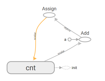
图为上述。cnt+a得到y,y通过assign赋值给cnt。
运行过程中,初始化变量后,通过每次运行assign,即完成了输出效果:1,2,3
config=tf.ConfigProto(allow_soft_placement=True)
cnt=tf.Variable(0,name="cnt")
a=tf.constant(1,name="a")
y=tf.add(cnt,a)
y2=tf.assign(cnt,y)
init=tf.initialize_all_variables()
with tf.Session(config=config) as ss:
    ss.run(init)
    xss=ss.run(cnt)
    for xc in range(3):
        ys2=ss.run(y2)
        print(ys2)
    xsum=tf.summary.FileWriter(".",ss.graph)
点乘数据
可以使用一维,二维,等进行点乘,只要数据对应即可。使用feed_dict进行数据输入。run后的返回值即为数据输出。
a=tf.placeholder(tf.float32,name='ta')
b=tf.placeholder(tf.float32,name='tb')
c=tf.multiply(a,b,name='tc')
config=tf.ConfigProto(allow_soft_placement=True)
init=tf.initialize_all_variables()
with tf.Session(config=config) as ss:
    ss.run(init)
    xss=ss.run([c],feed_dict={a:[7,2],b:[2,2]})
    print(xss)
    xsum=tf.summary.FileWriter(".",ss.graph)
也可写成如下形式:将变量分离出来定义。
a=tf.placeholder(tf.float32,name='ta')
b=tf.placeholder(tf.float32,name='tb')
c=tf.multiply(a,b,name='tc')
config=tf.ConfigProto(allow_soft_placement=True)
init=tf.initialize_all_variables()
a_data=[[1,2,3],[4,5,6]]
b_data=[[2,3,4],[5,6,7]]
with tf.Session(config=config) as ss:
    ss.run(init)
    xss=ss.run([c],feed_dict={a:a_data,b:b_data})
    print(xss)
    xsum=tf.summary.FileWriter(".",ss.graph)
run过程的一些写法
书写过程中,可以使用中括号,然后输出(本次输出为【7,21】)
a=tf.constant(3,name='ta')
b=tf.constant(2,name='tb')
c=tf.constant(5,name='tc')
m1=tf.add(b,c,name='m1')
m2=tf.multiply(a,m1,name='m2')
config=tf.ConfigProto(allow_soft_placement=True)
with tf.Session(config=config) as ss:
    xss=ss.run([m1,m2])
    print(xss)
    xsum=tf.summary.FileWriter(".",ss.graph)
也可以如下所代表的批量输出:
y2,w2,l2=ss.run(y),ss.run(w),ss.run(loss)
构建单神经元的神经网络
y=w*x
loss=(y-y_)^2
使用学习率为0.025的梯度下降,最小化loss。
定义完模型后,通过tf.summary.scalar控制tensorboard输出scalar数据图,显示数据的变化情况。
然后进行运算,最终的结果,通过saver=tf.train.Saver()的一些方法保存模型(训练后的模型)
w=tf.Variable(0.8,name='weight')
x=tf.constant(2.0,name='input')
y=tf.multiply(w,x,name='output')
y_=tf.constant(0.0,name='correct_value')
loss=tf.pow(y-y_,2,name='loss')
train_step=tf.train.GradientDescentOptimizer(0.025).minimize(loss)

with tf.name_scope('summar'):
    for value in [x,w,y,y_,loss]:
        tf.summary.scalar(value.op.name,value)
    #tf.summary.histogram('histogram',w)
    #tf.summary.histogram('loss',loss)
    summaries=tf.summary.merge_all()

config=tf.ConfigProto(allow_soft_placement=True)
init=tf.initialize_all_variables()

with tf.Session(config=config) as ss:
    xsum=tf.summary.FileWriter(".",ss.graph)
    xss=ss.run(init)
    for i in range(100):
        x_data=ss.run(summaries)
        xsum.add_summary(x_data,i)
        x_data=ss.run(train_step)
        y2,w2,l2=ss.run(y),ss.run(w),ss.run(loss)
        print(i,' ',y2,' ',w2,' ',l2,' ')
    saver=tf.train.Saver()
    saver.save(ss,'tmp/.')
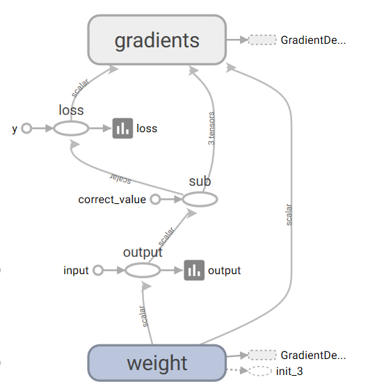

构建的张量图如上,点击其中的一些空心圆,可以查看其数值,操作,在gradient模块中,点开可以看到内部详细的结构。
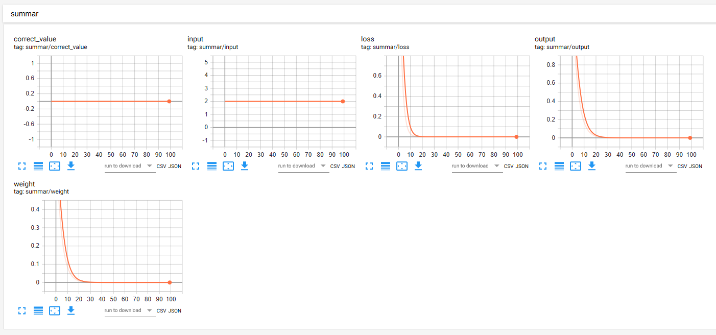
通过上述代码,在summer中归并了一些scalar图如下:
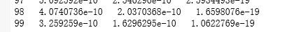
在迭代100次后,输出为:
模型保存读取
参阅:https://blog.csdn.net/Tan_HandSome/article/details/79303269
认为有两个文件保存,一个是meta文件保存模型,一个是checkpoint文件保存变量。至于其他文件的更新和变动还没有考虑。
下面一例:
使用w4=w3*b1
其中w3=w1+w2
实际保存的模型是这样,实际保存的变量,除掉placeholder占位符,只有b1=2一个值。
import tensorflow as tf
#Prepare to feed input, i.e. feed_dict and placeholders
w1 = tf.placeholder("float", name="w1")
w2 = tf.placeholder("float", name="w2")
b1= tf.Variable(2.0,name="bias")
feed_dict ={w1:4,w2:8}
#Define a test operation that we will restore
w3 = tf.add(w1,w2)
w4 = tf.multiply(w3,b1,name="op_to_restore")
sess = tf.Session()
sess.run(tf.global_variables_initializer())
#Create a saver object which will save all the variables
saver = tf.train.Saver()
#Run the operation by feeding input
print(sess.run(w4,feed_dict))
#Prints 24 which is sum of (w1+w2)*b1
#Now, save the graph
saver.save(sess, './save/my_test_model',global_step=1000)
另外开一个程序,运行如下:
因为b1保存了,所以这里占位符输入了13,17,然后计算的结果就是30*2了。
import tensorflow as tf
sess=tf.Session()
#First let's load meta graph and restore weights
saver = tf.train.import_meta_graph('my_test_model-1000.meta')

saver.restore(sess,tf.train.latest_checkpoint('./'))

# Now, let's access and create placeholders variables and
# create feed-dict to feed new data
graph = tf.get_default_graph()
w1 = graph.get_tensor_by_name("w1:0")
w2 = graph.get_tensor_by_name("w2:0")
feed_dict ={w1:13.0,w2:17.0}
#Now, access the op that you want to run.
op_to_restore = graph.get_tensor_by_name("op_to_restore:0")
print(sess.run(op_to_restore,feed_dict))
#This will print 60 which is calculated
#using new values of w1 and w2 and saved value of b1.