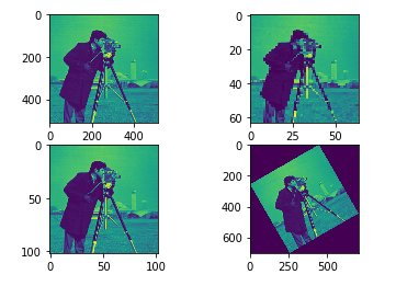
图像的重定义大小,图像的缩扩,图像的旋转:
 1 from skimage import transform,data
 2 import matplotlib.pyplot as plt
 3 img = data.camera()
 4 print(img.shape)
 5 plt.subplot(221)
 6 plt.imshow(img)
 7 plt.subplot(222)
 8 plt.imshow(transform.resize(img,(64,64)))
 9 plt.subplot(223)
10 plt.imshow(transform.rescale(img,0.2))
11 plt.subplot(224)
12 plt.imshow(transform.rotate(img,30,resize=True))
13 plt.show()
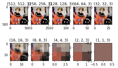
产生高斯金字塔
 1 import numpy as np
 2 import matplotlib.pyplot as plt
 3 from skimage import data,transform
 4 image = data.astronaut()  #载入宇航员图片
 5 pyramid = transform.pyramid_gaussian(image, downscale=2)  #产生高斯金字塔图像
 6 #pyramid = transform.pyramid_laplacian(image, downscale=2)
 7 #共生成了log(512)=9幅金字塔图像,加上原始图像共10幅,pyramid[0]-pyramid[1]
 8 i = 1
 9 for p in pyramid:
10     plt.subplot(2,5,i)
11     i+=1
12     #p[:,:,:]*=255
13     plt.title(p.shape)
14     plt.imshow(p)
15 plt.show()
gamma调整原理:I=Ig 如果gamma>1, 新图像比原图像暗。如果gamma<1,新图像比原图像亮
log对数调整I=log(I)
对比度是否偏低判断:exposure.is_low_contrast(img)
 1 from skimage import data, exposure, img_as_float
 2 import matplotlib.pyplot as plt
 3 image = img_as_float(data.moon())
 4 gam1= exposure.adjust_gamma(image, 4)   #调暗
 5 gam2= exposure.adjust_gamma(image, 0.7)  #调亮
 6 gam3= exposure.adjust_log(image)   #对数调整
 7 plt.figure('adjust_gamma',figsize=(10,10))
 8 plt.subplot(141)
 9 plt.imshow(image)
10 plt.subplot(142)
11 plt.imshow(gam1)
12 plt.subplot(143)
13 plt.imshow(gam2,plt.cm.gray)
14 plt.subplot(144)
15 plt.imshow(gam3)
16 plt.show()   #原理:I=Ig
17 result=exposure.is_low_contrast(gam1)
18 result
调整图片强度,不是很懂参数...
 1 import numpy as np
 2 from skimage import exposure
 3 image = data.moon()
 4 mat=exposure.rescale_intensity(image,out_range=(0,100))
 5 plt.subplot(121)
 6 plt.imshow(mat)
 7 print(image)
 8 print(mat)
 9 mat1=exposure.rescale_intensity(image, in_range=(0, 200))
10 plt.subplot(122)
11 plt.imshow(mat1)
12 print(mat1.min())
13 print(mat1)
绘制直方图
1 from skimage import data
2 import matplotlib.pyplot as plt
3 img=data.camera()
4 plt.figure("hist")
5 arr=img.flatten()
6 n, bins, patches = plt.hist(arr, bins=256, normed=1,facecolor='red')
7 plt.show()

彩色图片三通道直方图:
 1 from skimage import data
 2 import matplotlib.pyplot as plt
 3 img=data.astronaut()
 4 ar=img[:,:,0].flatten()
 5 plt.hist(ar, bins=256, normed=1,facecolor='r',edgecolor='r',hold=1)
 6 ag=img[:,:,1].flatten()
 7 plt.hist(ag, bins=256, normed=1, facecolor='g',edgecolor='g',hold=1)
 8 ab=img[:,:,2].flatten()
 9 plt.hist(ab, bins=256, normed=1, facecolor='b',edgecolor='b')
10 plt.show()
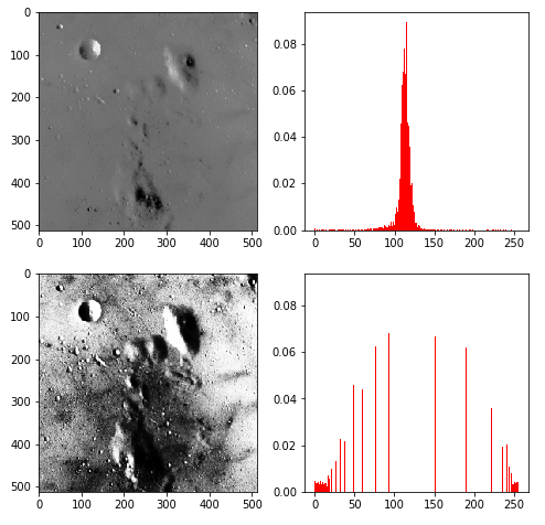
直方图均衡化exposure.equalize_hist(img)
对图像中像素个数多的灰度级进行展宽,而对图像中像素个数少的灰度进行压缩,从而扩展取值的动态范围,提高了对比度和灰度色调的变化,使图像更加清晰。
 1 from skimage import data,exposure
 2 import matplotlib.pyplot as plt
 3 img=data.moon()
 4 plt.figure("hist",figsize=(8,8))
 5
 6 arr=img.flatten()
 7 plt.subplot(221)
 8 plt.imshow(img,plt.cm.gray)  #原始图像
 9 plt.subplot(222)
10 plt.hist(arr, bins=256, normed=1,edgecolor='None',facecolor='red') #原始图像直方图
11
12 img1=exposure.equalize_hist(img)
13 arr1=img1.flatten()
14 plt.subplot(223)
15 plt.imshow(img1,plt.cm.gray)  #均衡化图像
16 plt.subplot(224)
17 arr1*=255
18 plt.hist(arr1, bins=256, normed=1,edgecolor='None',facecolor='red') #均衡化直方图
19
20 plt.show()
图像滤波:
平滑滤波,用来抑制噪声;微分算子,可以用来检测边缘和特征提取。
sobel、roberts、scharr、prewitt、canny算子
gabor、gaussian、median滤波
水平、垂直边缘检测
正负交叉边缘检测
 1 from skimage import data,filters,feature
 2 import matplotlib.pyplot as plt
 3 from skimage.morphology import disk
 4 img = data.camera()
 5 edges = filters.sobel(img)
 6 edges = filters.roberts(img)
 7 edges = filters.scharr(img)
 8 edges = filters.prewitt(img)
 9 edges = feature.canny(img,sigma=3)
10 edges,filt_imag  = filters.gabor(img, frequency=0.5)
11 edges = filters.gaussian(img,sigma=5)
12 edges = filters.median(img,disk(9))
13 edges = filters.sobel_h(img)
14 #水平边缘检测:sobel_h, prewitt_h, scharr_h
15 #垂直边缘检测: sobel_v, prewitt_v, scharr_v
16 edges = filters.roberts_neg_diag(img)
17 edges = filters.roberts_pos_diag(img)
18 plt.imshow(edges,plt.cm.gray)
图像阈值判断与分割的各种方法:
 1 from skimage import data,filters
 2 import matplotlib.pyplot as plt
 3 image = data.camera()
 4 thresh = filters.threshold_otsu(image)
 5 thresh = filters.threshold_yen(image)
 6 thresh = filters.threshold_li(image)
 7 thresh = filters.threshold_isodata(image)
 8
 9 dst =(image <= thresh)*1.0   #根据阈值进行分割
10 #dst =filters.threshold_adaptive(image, 31,'mean')
11 plt.subplot(121)
12 plt.title('original image')
13 plt.imshow(image,plt.cm.gray)
14 plt.subplot(122)
15 plt.title('binary image')
16 plt.imshow(dst,plt.cm.gray)
17 plt.show()

图形的绘制,与颜色。有各种各样的图形啊...
1 from skimage import draw,data
2 import matplotlib.pyplot as plt
3 img=data.chelsea()
4 rr, cc=draw.ellipse(150, 150, 30, 80)   #返回像素坐标
5 draw.set_color(img,[rr,cc],[255,0,0])
6 plt.imshow(img,plt.cm.gray)

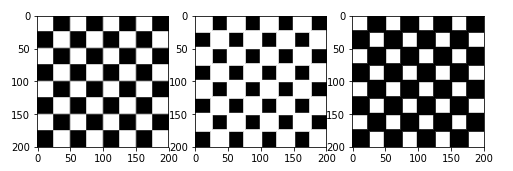
图像的膨胀,腐蚀
 1 from skimage import data
 2 import skimage.morphology as sm
 3 import matplotlib.pyplot as plt
 4 img=data.checkerboard()
 5 dst=sm.dilation(img,sm.square(5))  #用边长为15的正方形滤波器进行膨胀滤波
 6 dst1=sm.erosion(img,sm.square(5))  #用边长为5的正方形滤波器进行膨胀滤波
 7 plt.figure(figsize=(8,8))
 8 plt.subplot(131)
 9 plt.imshow(img,plt.cm.gray)
10 plt.subplot(132)
11 plt.imshow(dst,plt.cm.gray)
12 plt.subplot(133)
13 plt.imshow(dst1,plt.cm.gray)
14 #找到像素值为1的点,将它的邻近像素点都设置成这个值。1值表示白,0值表示黑,因此膨胀操作可以扩大白色值范围,压缩黑色值范围。一般用来扩充边缘或填充小的孔洞
15 #将0值扩充到邻近像素。扩大黑色部分,减小白色部分。可用来提取骨干信息,去掉毛刺,去掉孤立的像素。
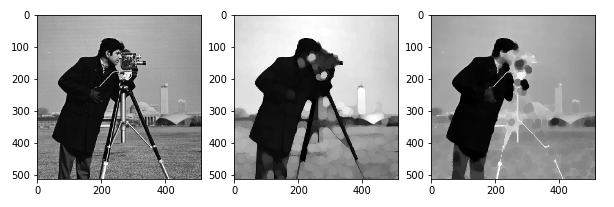
图像开运算,图像闭运算:
 1 from skimage import io,color,data
 2 import skimage.morphology as sm
 3 import matplotlib.pyplot as plt
 4 img=color.rgb2gray(data.camera())
 5 dst=sm.opening(img,sm.disk(9))  #用边长为9的圆形滤波器进行膨胀腐蚀滤波
 6 dst1=sm.closing(img,sm.disk(9))  #用边长为5的圆形滤波器进行腐蚀膨胀滤波
 7 plt.figure(figsize=(10,10))
 8 plt.subplot(131)
 9 plt.imshow(img,plt.cm.gray)
10 plt.subplot(132)
11 plt.imshow(dst,plt.cm.gray)
12 plt.subplot(133)
13 plt.imshow(dst1,plt.cm.gray)
白帽(white-tophat)。黑帽(black-tophat)。
 1 from skimage import io,color
 2 import skimage.morphology as sm
 3 import matplotlib.pyplot as plt
 4 img=color.rgb2gray(data.camera())
 5 dst=sm.white_tophat(img,sm.square(21))  #将原图像减去它的开运算值,返回比结构化元素小的白点
 6 dst1=sm.black_tophat(img,sm.square(21))  #将原图像减去它的闭运算值,返回比结构化元素小的黑点,且将这些黑点反色。
 7 plt.figure('morphology',figsize=(10,10))
 8 plt.subplot(131)
 9 plt.imshow(img,plt.cm.gray)
10 plt.subplot(132)
11 plt.imshow(dst,plt.cm.gray)
12 plt.subplot(133)
13 plt.imshow(dst1,plt.cm.gray)