Destruction and Construction Learning for Fine-grained Image Recognition
Intro
本文提出一种细粒度图像分类的方法,即将原图像拼图一样shuffle成不同的block,丢进一个分类器,当然,直接这样训练会引入shuffle带来的无关噪声,所以又加上了adversarial learning和construction learning,类比自编码器,其实这样的操作是使得网络学习到的feature map更加贴近正常图片的feature map,防止网络输出的feature map引入过多的噪声,从而关注真正对细粒度分类有用的部分。整个过程相当于用三个放大镜,层层筛选,筛选得到不管怎么shuffle都对细粒度分类有用的特征。
整个网络的结构如下图所示,清晰明了:
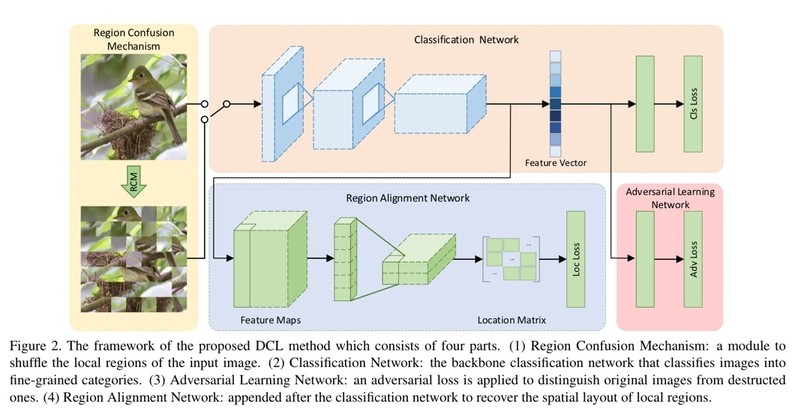
Region Confusion Mechanism
这一部分是“拼图”打乱的过程。
文章中对该部分的描述比较模糊,我看了一下没怎么看懂,就直接取找了一下源码,看了一下源码瞬间就秒懂了。
首先将原图划分为NxN个patch,然后遍历每个patch,遍历每个patch时,将行patch的该位置减k到该位置所有的patch shuffle,然后将列patch做同样的操作,直到遍历完所有像素。细节见代码,毕竟talk is cheap:
def swap(img, crop):
    def crop_image(image, cropnum):
        width, high = image.size
        crop_x = [int((width / cropnum[0]) * i) for i in range(cropnum[0] + 1)]
        crop_y = [int((high / cropnum[1]) * i) for i in range(cropnum[1] + 1)]
        im_list = []
        for j in range(len(crop_y) - 1):
            for i in range(len(crop_x) - 1):
                im_list.append(image.crop((crop_x[i], crop_y[j], min(crop_x[i + 1], width), min(crop_y[j + 1], high))))
        return im_list

    widthcut, highcut = img.size
    img = img.crop((10, 10, widthcut-10, highcut-10))
    images = crop_image(img, crop)
    pro = 5
    if pro >= 5:
        tmpx = []
        tmpy = []
        count_x = 0
        count_y = 0
        k = 1
        RAN = 2
        for i in range(crop[1] * crop[0]):
            tmpx.append(images[i])
            count_x += 1
            if len(tmpx) >= k:
                tmp = tmpx[count_x - RAN:count_x]
                random.shuffle(tmp)
                tmpx[count_x - RAN:count_x] = tmp
            if count_x == crop[0]:
                tmpy.append(tmpx)
                count_x = 0
                count_y += 1
                tmpx = []
            if len(tmpy) >= k:
                tmp2 = tmpy[count_y - RAN:count_y]
                random.shuffle(tmp2)
                tmpy[count_y - RAN:count_y] = tmp2
        random_im = []
        for line in tmpy:
            random_im.extend(line)

        # random.shuffle(images)
        width, high = img.size
        iw = int(width / crop[0])
        ih = int(high / crop[1])
        toImage = Image.new('RGB', (iw * crop[0], ih * crop[1]))
        x = 0
        y = 0
        for i in random_im:
            i = i.resize((iw, ih), Image.ANTIALIAS)
            toImage.paste(i, (x * iw, y * ih))
            x += 1
            if x == crop[0]:
                x = 0
                y += 1
    else:
        toImage = img
    toImage = toImage.resize((widthcut, highcut))
    return toImage
Adversarial Learning
如上所说,对抗训练的目的是为了给网络加一层约束,即让网络学习到的特征能够过滤掉shuffle带来的noise,从而学习到对细粒度分类更加有帮助的特征。
因此只需要一个二分类判别器来判断图像是否真实即可,其loss可写为:
其中(I)表述输入图像,D为二分类神经网络,( extbf{d}_I)表示gt的one-hot表示,(phi)表示RCM操作。
上式相当于是两个二分类交叉熵的和,因为公式是对正例和负例同时做的(因为可以直接得到两个),所以求和很好理解。
Construction Learning
与上面对抗训练一样,重建支路带来的梯度回传同样可以指导网络学习更加有用的feature,这在很多paper都用到了,讨论班的时候也听学长们讲过。
该部分的设计是使得网络学习将结构后的feature map映射到原来没有RCM的位置,也就是patch的下标。因此,重构网络的输出必须是(2 cdot N cdot N)的,文章的做法是先接一个1×1 conv将结构网络输出的feature map 转化为channel为2的feature map,然后relu+pooling,使得网络的输出刚好为(2cdot N cdot N)的。
其Loss定义为:
其中,(sigma(i,j))表示(i,j)经过RCM变换后的位置M表述重构网络,(M_{(i,j)})表示取重构网络输出结果的第(i,j)个向量,因为该处的feature对应的应该是未经过RCM的原图的(i,j)位置,所以两者的target都是(i,j).
最终联合训练的loss为: