iris数据集预测(对比随机森林和逻辑回归算法)
随机森林
library(randomForest)
#挑选响应变量
index <- subset(iris,Species != "setosa")
ir <- droplevels(index)
set.seed(1)
ind<-sample(2,nrow(ir),replace=TRUE,prob=c(0.7,0.3))
train<-ir[ind==1,]
test<-ir[ind==2,]
rf<-randomForest(Species~.,data=train,ntree=100)
rf

Call:
 randomForest(formula = Species ~ ., data = train, ntree = 100)
               Type of random forest: classification
                     Number of trees: 100
No. of variables tried at each split: 2

        OOB estimate of  error rate: 5.88%
Confusion matrix:
           versicolor virginica class.error
versicolor         32         2  0.05882353
virginica           2        32  0.05882353
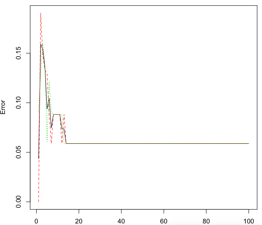
#随机森林的误差率
plot(rf)
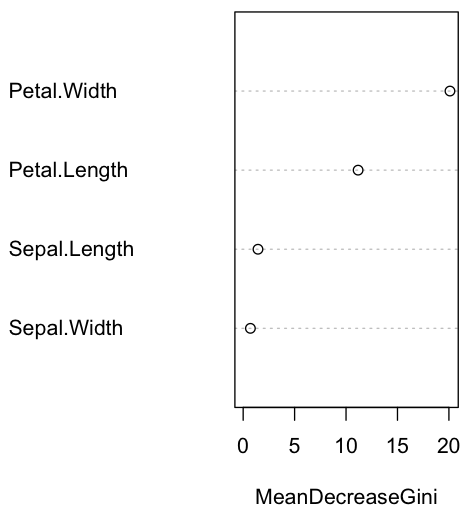
#变量重要性
importance(rf)
importance(rf)
             MeanDecreaseGini
Sepal.Length        1.4398647
Sepal.Width         0.7037353
Petal.Length       11.1734509
Petal.Width        20.1025569
varImpPlot(rf)
#查看预测结果
pred<-predict(rf,newdata=test)
table(pred,test$Species)

pred         versicolor virginica
  versicolor         15         2
  virginica           1        14
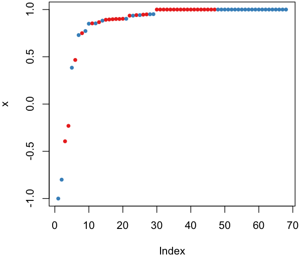
#预测边距
plot(margin(rf,test$Species))
逻辑回归
library(pROC)
g1<-glm(Species~.,family=binomial(link='logit'),data=train)
pre1<-predict(g1,type="response")
g1

Call:  glm(formula = Species ~ ., family = binomial(link = "logit"),
    data = train)

Coefficients:
 (Intercept)  Sepal.Length   Sepal.Width  Petal.Length   Petal.Width
   -32.01349      -3.85855      -0.02084       6.65355      14.08817

Degrees of Freedom: 67 Total (i.e. Null);  63 Residual
Null Deviance:        94.27
Residual Deviance: 8.309     AIC: 18.31

summary(g1)

Call:
glm(formula = Species ~ ., family = binomial(link = "logit"),
    data = train)

Deviance Residuals:
     Min        1Q    Median        3Q       Max
-1.73457  -0.02241  -0.00011   0.03691   1.76243

Coefficients:
              Estimate Std. Error z value Pr(>|z|)
(Intercept)  -32.01349   28.51193  -1.123   0.2615
Sepal.Length  -3.85855    3.16430  -1.219   0.2227
Sepal.Width   -0.02084    4.85883  -0.004   0.9966
Petal.Length   6.65355    5.47953   1.214   0.2246
Petal.Width   14.08817    7.32507   1.923   0.0544 .
---
Signif. codes:  0 '***' 0.001 '**' 0.01 '*' 0.05 '.' 0.1 ' ' 1

(Dispersion parameter for binomial family taken to be 1)

    Null deviance: 94.268  on 67  degrees of freedom
Residual deviance:  8.309  on 63  degrees of freedom
AIC: 18.309

Number of Fisher Scoring iterations: 9
#方差分析
anova(g1,test="Chisq")
Analysis of Deviance Table

Model: binomial, link: logit

Response: Species

Terms added sequentially (first to last)


             Df Deviance Resid. Df Resid. Dev  Pr(>Chi)
NULL                            67     94.268
Sepal.Length  1   14.045        66     80.223 0.0001785 ***
Sepal.Width   1    0.782        65     79.441 0.3764212
Petal.Length  1   62.426        64     17.015 2.766e-15 ***
Petal.Width   1    8.706        63      8.309 0.0031715 **
---
Signif. codes:  0 '***' 0.001 '**' 0.01 '*' 0.05 '.' 0.1 ' ' 1
#计算最优阀值
modelroc1<-roc(as.factor(ifelse(train$Species=="virginica",1,0)),pre1)
plot(modelroc1,print.thres=TRUE)

评估模型的预测效果
predict <-predict(g1,type="response",newdata=test)
predict.results <-ifelse(predict>0.804,"virginica","versicolor")
misClasificError <-mean(predict.results !=test$Species)
print(paste("Accuracy:",1-misClasificError))
[1] "Accuracy: 0.90625"
XGBoost
y<-data.matrix(as.data.frame(train$Species))-1
x<-data.matrix(train[-5])
bst <- xgboost(data =x, label = y, max.depth = 2, eta = 1,nround = 2, objective = "binary:logistic")

[1]    train-error:0.029412
[2]    train-error:0.029412
p<-predict(bst,newdata=data.matrix(test))
modelroc2<-roc(as.factor(ifelse(test$Species=="virginica",1,0)),p)
plot(modelroc2)

predict.results <-ifelse(p>0.11,"virginica","versicolor")
misClasificError <-mean(predict.results !=test$Species)
print(paste(1-misClasificError))
[1] "0.90625"