员工离职预测
library(dplyr)
library(psych)
library(ggplot2)
library(randomForest)
str(train)
'data.frame':    1100 obs. of  31 variables:
 $ X...Age                 : int  37 54 34 39 28 24 29 36 33 34 ...
 $ Attrition               : int  0 0 1 0 1 0 0 0 0 0 ...
 $ BusinessTravel          : Factor w/ 3 levels "Non-Travel","Travel_Frequently",..: 3 2 2 3 2 3 3 3 3 3 ...
 $ Department              : Factor w/ 3 levels "Human Resources",..: 2 2 2 2 2 3 2 3 2 2 ...
 $ DistanceFromHome        : int  1 1 7 1 1 4 9 2 4 2 ...
 $ Education               : int  4 4 3 1 3 1 5 2 4 4 ...
 $ EducationField          : Factor w/ 6 levels "Human Resources",..: 2 2 2 2 4 4 5 4 4 6 ...
 $ EmployeeNumber          : int  77 1245 147 1026 1111 1445 455 513 305 1383 ...
 $ EnvironmentSatisfaction : int  1 4 1 4 1 4 2 2 3 3 ...
 $ Gender                  : Factor w/ 2 levels "Female","Male": 2 1 2 1 2 1 2 2 1 1 ...
 $ JobInvolvement          : int  2 3 1 2 2 3 2 2 2 3 ...
 $ JobLevel                : int  2 3 2 4 1 2 1 3 1 2 ...
 $ JobRole                 : Factor w/ 9 levels "Healthcare Representative",..: 5 5 3 5 3 8 3 8 7 1 ...
 $ JobSatisfaction         : int  3 3 3 4 2 3 4 3 2 4 ...
 $ MaritalStatus           : Factor w/ 3 levels "Divorced","Married",..: 1 1 3 2 1 2 3 2 2 3 ...
 $ MonthlyIncome           : int  5993 10502 6074 12742 2596 4162 3983 7596 2622 6687 ...
 $ NumCompaniesWorked      : int  1 7 1 1 1 1 0 1 6 1 ...
 $ Over18                  : Factor w/ 1 level "Y": 1 1 1 1 1 1 1 1 1 1 ...
 $ OverTime                : Factor w/ 2 levels "No","Yes": 1 1 2 1 1 2 1 1 1 1 ...
 $ PercentSalaryHike       : int  18 17 24 16 15 12 17 13 21 11 ...
 $ PerformanceRating       : int  3 3 4 3 3 3 3 3 4 3 ...
 $ RelationshipSatisfaction: int  3 1 4 3 1 3 3 2 4 4 ...
 $ StandardHours           : int  80 80 80 80 80 80 80 80 80 80 ...
 $ StockOptionLevel        : int  1 1 0 1 2 2 0 2 0 0 ...
 $ TotalWorkingYears       : int  7 33 9 21 1 5 4 10 7 14 ...
 $ TrainingTimesLastYear   : int  2 2 3 3 2 3 2 2 3 2 ...
 $ WorkLifeBalance         : int  4 1 3 3 3 3 3 3 3 4 ...
 $ YearsAtCompany          : int  7 5 9 21 1 5 3 10 3 14 ...
 $ YearsInCurrentRole      : int  5 4 7 6 0 4 2 9 2 11 ...
 $ YearsSinceLastPromotion : int  0 1 0 11 0 0 2 9 1 4 ...
 $ YearsWithCurrManager    : int  7 4 6 8 0 3 2 0 1 11 ...
describe(train)
                          vars    n    mean      sd median trimmed     mad  min   max range  skew kurtosis     se
X...Age                     1 1100   37.00    9.04   36.0   36.51    8.90   18    60    42  0.44    -0.43   0.27
Attrition                   2 1100    0.16    0.37    0.0    0.08    0.00    0     1     1  1.83     1.36   0.01
BusinessTravel*             3 1100    2.62    0.66    3.0    2.77    0.00    1     3     2 -1.47     0.81   0.02
Department*                 4 1100    2.26    0.52    2.0    2.25    0.00    1     3     2  0.23    -0.41   0.02
DistanceFromHome            5 1100    9.43    8.20    7.0    8.36    7.41    1    29    28  0.91    -0.35   0.25
Education                   6 1100    2.92    1.02    3.0    2.99    1.48    1     5     4 -0.30    -0.55   0.03
EducationField*             7 1100    3.22    1.32    3.0    3.06    1.48    1     6     5  0.58    -0.65   0.04
EmployeeNumber              8 1100 1028.16  598.92 1026.5 1027.04  782.81    1  2065  2064  0.02    -1.22  18.06
EnvironmentSatisfaction     9 1100    2.73    1.10    3.0    2.78    1.48    1     4     3 -0.33    -1.21   0.03
Gender*                    10 1100    1.59    0.49    2.0    1.62    0.00    1     2     1 -0.38    -1.86   0.01
JobInvolvement             11 1100    2.73    0.71    3.0    2.74    0.00    1     4     3 -0.54     0.34   0.02
JobLevel                   12 1100    2.05    1.11    2.0    1.89    1.48    1     5     4  1.04     0.40   0.03
JobRole*                   13 1100    5.43    2.46    6.0    5.59    2.97    1     9     8 -0.34    -1.22   0.07
JobSatisfaction            14 1100    2.73    1.11    3.0    2.79    1.48    1     4     3 -0.33    -1.24   0.03
MaritalStatus*             15 1100    2.11    0.73    2.0    2.14    1.48    1     3     2 -0.18    -1.12   0.02
MonthlyIncome              16 1100 6483.62 4715.29 4857.0 5639.41 3166.09 1009 19999 18990  1.38     1.04 142.17
NumCompaniesWorked         17 1100    2.68    2.51    2.0    2.35    1.48    0     9     9  1.03    -0.02   0.08
Over18*                    18 1100    1.00    0.00    1.0    1.00    0.00    1     1     0   NaN      NaN   0.00
OverTime*                  19 1100    1.28    0.45    1.0    1.22    0.00    1     2     1  0.99    -1.02   0.01
PercentSalaryHike          20 1100   15.24    3.63   14.0   14.85    2.97   11    25    14  0.79    -0.35   0.11
PerformanceRating          21 1100    3.15    0.36    3.0    3.07    0.00    3     4     1  1.93     1.72   0.01
RelationshipSatisfaction   22 1100    2.70    1.10    3.0    2.75    1.48    1     4     3 -0.29    -1.23   0.03
StandardHours              23 1100   80.00    0.00   80.0   80.00    0.00   80    80     0   NaN      NaN   0.00
StockOptionLevel           24 1100    0.79    0.84    1.0    0.67    1.48    0     3     3  0.95     0.34   0.03
TotalWorkingYears          25 1100   11.22    7.83   10.0   10.27    5.93    0    40    40  1.15     0.99   0.24
TrainingTimesLastYear      26 1100    2.81    1.29    3.0    2.74    1.48    0     6     6  0.50     0.49   0.04
WorkLifeBalance            27 1100    2.75    0.70    3.0    2.76    0.00    1     4     3 -0.60     0.47   0.02
YearsAtCompany             28 1100    7.01    6.22    5.0    5.94    4.45    0    37    37  1.81     4.01   0.19
YearsInCurrentRole         29 1100    4.21    3.62    3.0    3.83    4.45    0    18    18  0.95     0.61   0.11
YearsSinceLastPromotion    30 1100    2.23    3.31    1.0    1.49    1.48    0    15    15  1.94     3.30   0.10
YearsWithCurrManager       31 1100    4.12    3.60    3.0    3.76    4.45    0    17    17  0.86     0.26   0.11
#删除 常量
name<-names(train)
train<-train[name!="Over18" & name!="StandardHours" & name!="EmployeeNumber"]
#重编码
train$Gender<-as.integer(train$Gender)-1
train$OverTime<-as.integer(train$OverTime)-1
#Age 和 Attrition
 ggplot(train, aes(X...Age, fill = factor(Attrition))) +
   geom_histogram(bins=30) +
   facet_grid(.~Gender)+
    labs(fill="Attrition")+ xlab("Age")+ylab("Total Count")

#小结:
train$X...Age[train$X...Age>=18 & train$X...Age <25]<-1
train$X...Age[train$X...Age>=25 & train$X...Age <35]<-2
train$X...Age[train$X...Age>=35 & train$X...Age <45]<-3
train$X...Age[train$X...Age>=45 & train$X...Age <55]<-4
train$X...Age[train$X...Age>=55 ]<-5
#Department 和 JobLevel
ggplot(train, aes(x = JobLevel, fill = as.factor(Attrition))) +
 geom_bar() +
 facet_wrap(~ Department)+

  xlab("Job Level")+

  ylab("Total Count")+

  labs(fill = "Attrition")

train$Department<-as.character(train$Department)
train$Department[train$Department=="Human Resources"]<-"1"
train$Department[train$Department=="Sales"]<-"2"
train$Department[train$Department=="Research & Development"]<-"3"
train$Department<-as.integer(train$Department)
#小结:不同部门相同级别之间存在明显差异,研发部门1,2级别和销售部1,2,3级别流动性较大。
#Department 和 BusinessTravel
ggplot(train, aes(x = BusinessTravel, fill = as.factor(Attrition))) +
   geom_bar() +
   facet_wrap(~ Department)+
   xlab("BusinessTravel")+
   ylab("Total Count")+
   labs(fill = "Attrition")

train$BusinessTravel<-as.character(train$BusinessTravel)
train$BusinessTravel[train$BusinessTravel=="Non-Travel"]<-"1"
train$BusinessTravel[train$BusinessTravel=="Travel_Frequently"]<-"2"
train$BusinessTravel[train$BusinessTravel=="Travel_Rarely"]<-"3"
train$BusinessTravel<-as.integer(train$BusinessTravel)
#小结:是否经常出差,并不是影响离职的关键因素,但偶然出差的员工离职率最高。研发部、销售部、人力资源部依次下降。
#EducationField 和 Attrition
ggplot(train,aes(EducationField,fill=as.factor(Attrition)))+
    geom_bar(stat="count",position="dodge")+
    xlab("EducationField")+
    ylab("Total Count")+
    labs(fill="Attrition")

#小结:专业领域和离职之间无明显关系
#MaritalStatus 和 Attrition
 ggplot(train,aes(MaritalStatus,fill=as.factor(Attrition)))+
     geom_bar(stat="count",position="dodge")+
     xlab("MaritalStatus")+
     ylab("Total Count")+
     labs(fill="Attrition")

train$MaritalStatus<-as.character(train$MaritalStatus)
train$MaritalStatus[train$MaritalStatus=="Divorced"]<-1
train$MaritalStatus[train$MaritalStatus=="Married"]<-2
train$MaritalStatus[train$MaritalStatus=="Single"]<-3
train$MaritalStatus<-as.integer(train$MaritalStatus)
#小结:婚姻情况和离职有一点关系
#EnvironmentSatisfaction 和 Attrition
ggplot(train, aes(x = EnvironmentSatisfaction, fill = as.factor(Attrition))) +
    geom_bar() +
    facet_wrap(~ JobLevel)+
    xlab("JobLevel")+
    ylab("Total Count")+
    labs(fill = "Attrition")

#小结:满意度和离职之间无明显关系
#MonthlyIncome 和 Attrition
ggplot(train,aes(MonthlyIncome, fill = factor(Attrition))) +
  geom_density(alpha = 0.8)+
  labs(fill="Attrition")
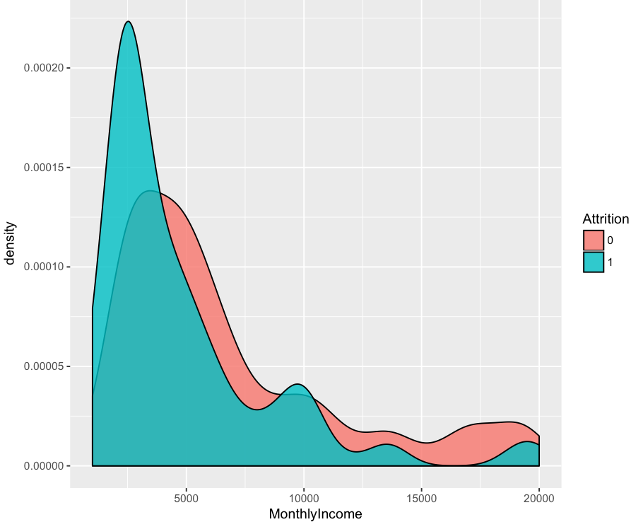
#小结:低收入者明显在职意向不稳定
train$MonthlyIncome[train$MonthlyIncome<=3000]<-1
train$MonthlyIncome[train$MonthlyIncome>3000 & train$MonthlyIncome<=6000]<-2
train$MonthlyIncome[train$MonthlyIncome>6000 & train$MonthlyIncome<=9000]<-3
train$MonthlyIncome[train$MonthlyIncome>9000 & train$MonthlyIncome<=12000]<-4
train$MonthlyIncome[train$MonthlyIncome>12000 & train$MonthlyIncome<=17000]<-5
train$MonthlyIncome[train$MonthlyIncome>17000]<-6
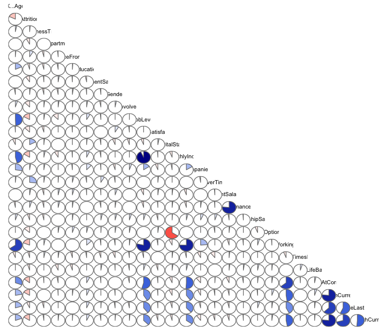
#关联关系
corrgram(train[,-c(7,12)],lower.panel=panel.pie,upper.panel=NULL)
#抽样
set.seed(1)
ind<-sample(2,nrow(train),replace=TRUE,prob=c(0.7,0.3))
train.df<-train[ind==1,]
test.df<-train[ind==2,]
#随机森林
rf<-randomForest(factor(Attrition)~.,data=train.df)
varImpPlot(rf)

#准确率
prediction <- predict(rf,newdata=test.df,type="response")
misClasificError <- mean(prediction != test.df$Attrition)
print(paste('Accuracy',1-misClasificError))
[1] "Accuracy 0.876506024096386"
#逻辑回归
gf<-glm(Attrition~.,data=train.df,family = binomial(link=logit))
summary(gf)

Call:
glm(formula = Attrition ~ ., family = binomial(link = logit),
    data = train.df)

Deviance Residuals:
    Min       1Q   Median       3Q      Max
-1.6113  -0.5048  -0.2459  -0.0860   3.4737

Coefficients:
                               Estimate Std. Error z value Pr(>|z|)
(Intercept)                    -1.31753    3.58064  -0.368 0.712903
X...Age                        -0.36136    0.17640  -2.049 0.040508 *
BusinessTravel                  0.05908    0.20110   0.294 0.768928
Department                      0.39070    0.93431   0.418 0.675820
DistanceFromHome                0.05274    0.01486   3.550 0.000386 ***
Education                      -0.17039    0.12279  -1.388 0.165239
EducationFieldLife Sciences    -0.43924    1.20639  -0.364 0.715785
EducationFieldMarketing         0.14995    1.25574   0.119 0.904948
EducationFieldMedical          -0.55928    1.20602  -0.464 0.642835
EducationFieldOther             0.07420    1.32247   0.056 0.955256
EducationFieldTechnical Degree  0.62904    1.22665   0.513 0.608084
EnvironmentSatisfaction        -0.50299    0.11646  -4.319 1.57e-05 ***
Gender                          0.49495    0.26618   1.859 0.062965 .
JobInvolvement                 -0.67266    0.17777  -3.784 0.000154 ***
JobLevel                       -0.18383    0.39279  -0.468 0.639777
JobRoleHuman Resources          2.92472    2.10883   1.387 0.165474
JobRoleLaboratory Technician    2.11121    0.82806   2.550 0.010785 *
JobRoleManager                  2.09557    1.12796   1.858 0.063193 .
JobRoleManufacturing Director   1.22695    0.84649   1.449 0.147211
JobRoleResearch Director        1.49258    1.17894   1.266 0.205501
JobRoleResearch Scientist       1.44543    0.82801   1.746 0.080868 .
JobRoleSales Executive          2.17131    1.20040   1.809 0.070479 .
JobRoleSales Representative     3.29933    1.28712   2.563 0.010367 *
JobSatisfaction                -0.63089    0.11767  -5.361 8.26e-08 ***
MaritalStatus                   0.94530    0.25146   3.759 0.000170 ***
MonthlyIncome                  -0.03459    0.24924  -0.139 0.889628
NumCompaniesWorked              0.13934    0.05418   2.572 0.010119 *
OverTime                        2.18546    0.27520   7.941 2.00e-15 ***
PercentSalaryHike              -0.05939    0.05572  -1.066 0.286492
PerformanceRating               0.86885    0.55923   1.554 0.120266
RelationshipSatisfaction       -0.33278    0.11625  -2.863 0.004201 **
StockOptionLevel                0.01585    0.21361   0.074 0.940835
TotalWorkingYears              -0.04047    0.04220  -0.959 0.337593
TrainingTimesLastYear          -0.15291    0.10058  -1.520 0.128425
WorkLifeBalance                -0.21648    0.16944  -1.278 0.201398
YearsAtCompany                  0.07885    0.05340   1.477 0.139745
YearsInCurrentRole             -0.13861    0.06449  -2.149 0.031612 *
YearsSinceLastPromotion         0.14022    0.05867   2.390 0.016857 *
YearsWithCurrManager           -0.11790    0.06483  -1.819 0.068956 .
---
Signif. codes:  0 '***' 0.001 '**' 0.01 '*' 0.05 '.' 0.1 ' ' 1

(Dispersion parameter for binomial family taken to be 1)

    Null deviance: 717.22  on 767  degrees of freedom
Residual deviance: 457.00  on 729  degrees of freedom
AIC: 535

Number of Fisher Scoring iterations: 6
#准确率
prediction <- predict(gf,newdata=test.df,type="response")
prediction <- ifelse(prediction > 0.5,1,0)
misClasificError <- mean(prediction != test.df$Attrition)
print(paste('Accuracy',1-misClasificError))
[1] "Accuracy 0.858433734939759"