test <- read.csv(file.choose())
train <- read.csv(file.choose())
#注意:字符串要带有双引号
#“Sex”字段类型转换/生成新的字段值(因子类型字段处理)
train$sex[train$Sex == "female"] <- 0
train$sex[train$Sex == "male"] <- 1

test$sex[test$Sex == "female"] <- 0
test$sex[test$Sex == "male"] <- 1
#“Embarked“字段转换/生成新的字段值(因子类型字段处理)
train$embarked[train$Embarked == "C"] <-1
train$embarked[train$Embarked == "Q"] <-2
train$embarked[train$Embarked == "S"] <-3

test$embarked[test$Embarked == "C"] <-1
test$embarked[test$Embarked == "Q"] <-2
test$embarked[test$Embarked == "S"] <-3
#拆分字段"Name",获取称谓
title_train <- as.character(train$Name)
title_train <- strsplit(title_train," ")

title_test <- as.character(test$Name)
title_test <- strsplit(title_test," ")
#生成新字段title
train$title <- train$Survived
train$title <- as.character(train$title)

test$title <- test$PassengerId
test$title <- as.character(test$PassengerId)
#提取姓名中的称呼字段"Name" Warning
for(i in 1:length(train$title)){
temp_num <- grep("\\.",title_train[[i]]);
#if else 完善结构,无意义
if(is.integer(temp_num)) {
train$title[i] <- title_train[[i]][temp_num];
}
else {
train$title[i] <- NA;
}
}
#定义需要删除的字段
temp_name <- names(train)
temp_delete <- c("Embarked","Name","Sex")
#循环删除字段
for(i in 1:length(temp_delete))
temp_name <- temp_name[-grep(temp_delete[i],temp_name)]
train_set <- train[temp_name]


for(i in 1:length(test$title)){
temp_num <- grep("\\.",title_test[[i]]);
#if else 完善结构,无意义
if(is.integer(temp_num)) {
test$title[i] <- title_test[[i]][temp_num];
}
else {
test$title[i] <- NA;
}
}
#定义需要删除的字段
temp_name <- names(test)
temp_delete <- c("Embarked","Name","Sex")
#循环删除字段
for(i in 1:length(temp_delete))
temp_name <- temp_name[-grep(temp_delete[i],temp_name)]
test_set <- test[temp_name]

#剔除多余列的优化方案
# n<-names(train)
# head(train_ [n [n !="title" & n!="sex" & n!="Fare" ] ] )
#2017-08-06
#数据处理的目标:字段是否可用,如何转化为可用字段
#Ticket 可以根据字段特征(长度+前几位数字、相同字幕),确定字段是否属于同类型(级别)
#缺失值处理,可以对train和test数据集合并后进行处理
#作图
#导出图片
#savePlot(filename = "",
# type = c("wmf", "emf", "png", "jpg", "jpeg", "bmp",
# "tif", "tiff", "ps", "eps", "pdf"),
# device = dev.cur(),
# restoreConsole = TRUE)
#性别和生存关系
#savePlot(filename = "",
# type = c("wmf", "emf", "png", "jpg", "jpeg", "bmp",
# "tif", "tiff", "ps", "eps", "pdf"),
# device = dev.cur(),
# restoreConsole = TRUE)

#登船位置与生存关系
#barplot(table(train_set$Survived,train_set$embarked),col=c("red","green"),args.legend = list(x = "topleft"),legend.text = c("0", "1"))

#年龄的统计量
summary(train$Age)
#Min. 1st Qu. Median Mean 3rd Qu. Max. NA's
#0.42 20.12 28.00 29.70 38.00 80.00 177
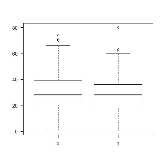
#箱线图查看生存和年龄的关系
#boxplot(Age~Survived, data=train)
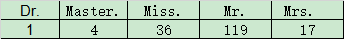
#查看年龄变量缺失值对应title统计量
table(train_set$title[is.na(train_set$Age)])
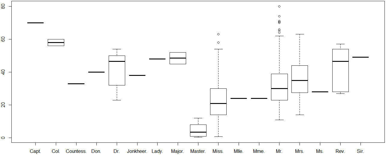
#查看train数据集中的title变量年龄的分布
#boxplot(Age~title,data=train_set)
#合并test和train数据集
train_age <- data.frame(train$Age,train$title)
names(train_age) <- c("age","title")
test_age <- data.frame(test$Age,test$title)
names(test_age) <- c("age","title")
combin_age <- rbind(train_age,test_age)
head(combind_age)
#剔除title出现次数较少行
temp <- combin_age[which(combin_age$title !="Capt."
& combin_age$title !="Countess."
& combin_age$title !="Don."
& combin_age$title !="Jonkheer."
& combin_age$title !="Lady."
& combin_age$title !="Mme."
& combin_age$title !="Sir."
& combin_age$title !="Dona."
& combin_age$title !="Ms."
& combin_age$title !="Mlle."
& combin_age$title !="Major."
& combin_age$title !="Col."
),]
#作图,合并后的age和title
#boxplot(age~title,data=temp)

#备份数据
train_ <- train_set
test_ <- test_set
#由于和年龄相关变量较少,故此处仅使用中位数作为缺失值
#获取年龄中位数
summary(temp[which(temp$title=="Dr."),]$age)
#Min. 1st Qu. Median Mean 3rd Qu. Max. NA's
#23.00 38.00 49.00 43.57 51.50 54.00 1
summary(temp[which(temp$title=="Master."),]$age)
#Min. 1st Qu. Median Mean 3rd Qu. Max. NA's
#0.330 2.000 4.000 5.483 9.000 14.500 8
summary(temp[which(temp$title=="Miss."),]$age)
#Min. 1st Qu. Median Mean 3rd Qu. Max. NA's
#0.17 15.00 22.00 21.77 30.00 63.00 50
summary(temp[which(temp$title=="Mr."),]$age)
#Min. 1st Qu. Median Mean 3rd Qu. Max. NA's
#11.00 23.00 29.00 32.25 39.00 80.00 176
summary(temp[which(temp$title=="Mrs."),]$age)
#Min. 1st Qu. Median Mean 3rd Qu. Max. NA's
#14.00 27.00 35.50 36.99 46.50 76.00 27
train_$Age[train_$title =="Miss." & is.na(train_$Age)]<-median(temp[which(temp$title=="Miss."),]$age,na.rm=TRUE)
train_$Age[train_$title =="Master." & is.na(train_$Age)]<-median(temp[which(temp$title=="Master."),]$age,na.rm=TRUE)
train_$Age[train_$title =="Mr." & is.na(train_$Age)]<-median(temp[which(temp$title=="Mr."),]$age,na.rm=TRUE)
train_$Age[train_$title =="Mrs." & is.na(train_$Age)]<-median(temp[which(temp$title=="Mrs."),]$age,na.rm=TRUE)
train_$Age[train_$title =="Dr." & is.na(train_$Age)]<-median(temp[which(temp$title=="Dr."),]$age,na.rm=TRUE)


test_$Age[test_$title =="Miss." & is.na(test_$Age)]<-median(temp[which(temp$title=="Miss."),]$age,na.rm=TRUE)
test_$Age[test_$title =="Master." & is.na(test_$Age)]<-median(temp[which(temp$title=="Master."),]$age,na.rm=TRUE)
test_$Age[test_$title =="Mr." & is.na(test_$Age)]<-median(temp[which(temp$title=="Mr."),]$age,na.rm=TRUE)
test_$Age[test_$title =="Mrs." & is.na(test_$Age)]<-median(temp[which(temp$title=="Mrs."),]$age,na.rm=TRUE)
test_$Age[test_$title =="Dr." & is.na(test_$Age)]<-median(temp[which(temp$title=="Dr."),]$age,na.rm=TRUE)
#剔除embarked为NA的行
train_ <- train_[!is.na(train_$embarked),]
test_ <- test_[!is.na(test_$embarked),]
#剔除多余的列
train_ <- train_[names(train_)[(names(train_) !="title")]]
test_ <- test_[names(test_)[(names(test_) !="title")]]
#票价有为0的
#从下图可以看出,船舱等级和票价之间的联系,然后对0票价进行处理
#summary(train_$Fare)
#发现存在票价为0的情况,查看为0的数量
#length(train_$Fare[train_$Fare == 0])
#剔除(未分析的)干扰项目
train_ <- train_[names(train_)[(names(train_) !="Cabin")]]
train_ <- train_[names(train_)[(names(train_) !="Ticket")]]

test_ <- test_[names(test_)[(names(test_) !="Cabin")]]
test_ <- test_[names(test_)[(names(test_) !="Ticket")]]
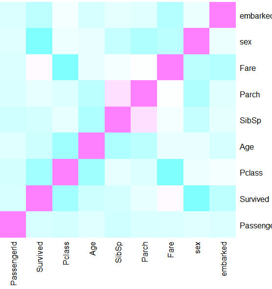
#查看变量直接的关联强度(剔除NA值)
#此处应该先把非定量序数变量变成定量序数变量后,采用Speaman进行相关分析
heatmap(cor(as.matrix(na.omit(train_))),symm = TRUE, Rowv=NA, Colv=NA, col = cm.colors(256))
#查看票价和船仓等级之间的关系
boxplot(Fare~Pclass,data=subset(train_,Fare != "512.3292"),horizontal=TRUE)
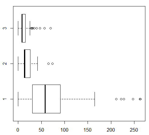
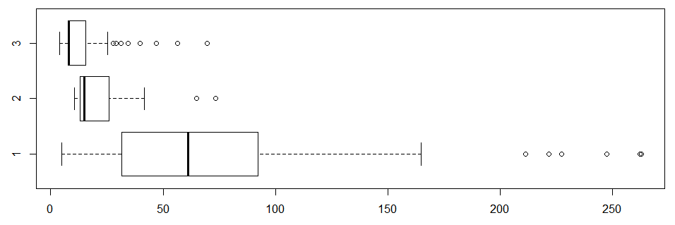
#剔除0值后再观察
boxplot(Fare~Pclass,data=subset(train_,Fare != "512.3292" & Fare !="0"),horizontal=TRUE)
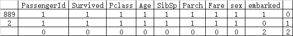
library(mice)
md.pattern(train_)
#用于熟悉分类方法,目前掌握的资料暂未发现使用该方法进行缺失值处理
#采用随机抽取的方法,把train_分为训练集和测试集
#分析两个模型
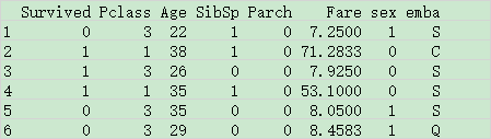
#获取到如下数据 head(newData)
#注意数据集中不能出现字符串,可以更改为因子
#指定百分比抽样数据,分作训练集和测试集
sampleData <- sample(2,replace= TRUE, nrow(newData), prob=c(0.7, 0.3))
trainData <- newData[sampleData==1,]
testData <- newData[sampleData==2,]
#条件推断树
library(party)
f1 <- emba ~ Survived + Pclass + Age + SibSp + Parch + Fare + sex
c_tree <- ctree(f1, data=trainData)
#绘制决策树
plot(c_tree)

#对测试数据进行预测
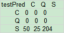
testPred <- predict(c_tree, newdata = testData)
table(testPred,testData$emba)
#随机森林方法进行预测
 library(randomForest)
 rf <- randomForest(f1, data=trainData, ntree=100, proximity=TRUE)
 table(predict(rf), trainData$emba)
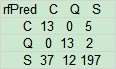
#由于预测效果极差,放弃该方法
#处理test中的NA的情况
#此处忽略操作......
f1<-glm(Survived~Pclass+Age+SibSp+Parch+Fare+sex+embarked,data=train_,family=binomial())

f2<-glm(Survived~Pclass+Age+SibSp+sex+embarked,data=train_,family=binomial())

anova(f1,f2,test="Chisq")

#Analysis of Deviance Table

#Model 1: Survived ~ Pclass + Age + SibSp + Parch + Fare + sex + embarked
#Model 2: Survived ~ Pclass + Age + SibSp + sex + embarked
#  Resid. Df Resid. Dev Df Deviance Pr(>Chi)
#1       881     781.22
#2       883     782.29 -2  -1.0685   0.5861
f3<-glm(Survived~Pclass+Age+SibSp+sex+embarked,data=train_,family=binomial())

test_p<-test_[,c("Pclass","Age","Fare","sex","embarked")]

pred<-predict(f3,test_p)

perf[perf>0]<-1

perf[perf<=0]<-0