以下是一些宏观要点:
神经网络是深度学习中非常流行的前沿技术;
深度学习是机器学习的分支;
机器学习是人工智能的分支;
深度学习包括四个主要概念。本文的目标是让读者掌握这四个深度学习基础概念:
前馈;
梯度下降;
全局最小值;
反向传播;
示例:
想象你是一家宠物店的老板,你通过下面一份调查问卷来预测顾客的购买行为!
1.您有猫吗?
2.您喝进口啤酒吗?
3.过去一个月,您是否访问过我们的网站 LitterRip.com?
4.过去一个月,您是否购买过 Litter Rip! 猫砂?
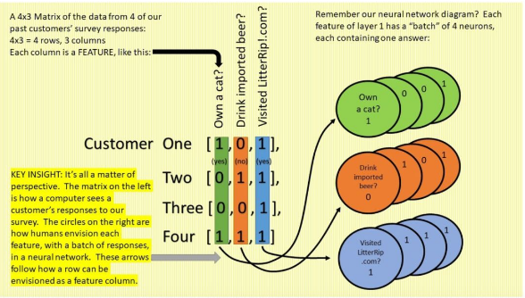
很显然【1,2,3】问题的答案作为神经网络的输入,【4】问题的答案作为输出。那么数据准备如下(共有四人参与调查问卷):
'''输入'''
[1,0,1],
[0,1,1],
[0,0,1],
[1,1,1]
'''输出'''
[1],
[1],
[0],
[0]
创建如下网络:
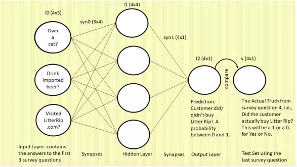
1.我们先来看这张图,图中是一个三层的前馈神经网络。左侧为输入层:三个圆圈表示神经元(即节点或特征,该网络将使用前三个调查问题作为特征)。现在,你看着这一列圆圈,想象它们分别代表一位顾客的答案。左上的圆圈包含问题 1「你有猫吗?」的答案,左中圆圈包含问题 2「你喝进口啤酒吗?」的答案,左下圆圈表示问题 3「你是否访问过我们的网站 LitterRip.com?」的答案。那么,如果顾客 1 对这三个问题的答案是「Yes/No/Yes」,则左上圆圈包含 1,左中圆圈包含 0,左下圆圈包含 1。这就与我们的数据集相对应了。
2.连接这些圆圈和隐藏层的所有线是神经网络用来「思考」的部位,也就是权重。右侧的单个圆圈(它依然和四个权重相连)是网络的预测结果,即「基于输入到网络的特征组合,此处展示了这位顾客购买新款猫砂的概率。」
3.最右侧标注「y」的单个圆圈表示真值,即每个顾客对第四个调查问题「你是否购买过 Litter Rip! 猫砂?」的回答。这个圆圈有两个选择:0 表示没买过,1 表示买过。神经网络将输出一个预测概率,并将其与 y 进行对比,查看准确率,然后在下一次迭代中吸取教训。神经网络在数秒时间内可以完成数万次试错。
4.对于输入数据下图给出了更形象的解释
先贴代码:
#This is the "3 Layer Network" near the bottom of:
#http://iamtrask.github.io/2015/07/12/basic-python-network/

#First, housekeeping: import numpy, a powerful library of math tools.
5 import numpy as np

#1 Sigmoid Function: changes numbers to probabilities and computes confidence to use in gradient descent
8 def nonlin(x,deriv=False):
9   if(deriv==True):
10    return x*(1-x)
11
12  return 1/(1+np.exp(-x))

#2 The X Matrix: This is the responses to our survey from 4 of our customers,
#in language the computer understands.  Row 1 is the first customer's set of
#Yes/No answers to the first 3 of our survey questions:
#"1" means Yes to, "Have cat who poops?" The "0" means No to "Drink imported beer?"
#The 1 for "Visited the LitterRip.com website?" means Yes.  There are 3 more rows
#(i.e., 3 more customers and their responses) below that.
#Got it?  That's 4 customers and their Yes/No responses
#to the first 3 questions (the 4th question is used in the next step below).
#These are the set of inputs that we will use to train our network.
23 X = np.array([[1,0,1],
24               [0,1,1],
25               [0,0,1],
26               [1,1,1]])
#3The y Vector: Our testing set of 4 target values. These are our 4 customers' Yes/No answers
#to question four of the survey, "Actually purchased Litter Rip?"  When our neural network
#outputs a prediction, we test it against their answer to this question 4, which
#is what really happened.  When our network's
#predictions compare well with these 4 target values, that means the network is
#accurate and ready to take on our second dataset, i.e., predicting whether our
#hot prospects from the (hot) veterinarian will buy Litter Rip!
34 y = np.array([[1],
35               [1],
36               [0],
37               [0]])
#4 SEED: This is housekeeping. One has to seed the random numbers we will generate
#in the synapses during the training process, to make debugging easier.
40 np.random.seed(1)
#5 SYNAPSES: aka "Weights." These 2 matrices are the "brain" which predicts, learns
#from trial-and-error, then improves in the next iteration.  If you remember the
#diagram of the curvy red bowl above, syn0 and syn1 are the
#X and Y axes on the white grid under the red bowl, so each time we tweak these
#values, we march the grid coordinates of Point A (think, "moving the yellow arrow")
#towards the red bowl's bottom, where error is near zero.
47 syn0 = 2*np.random.random((3,4)) - 1 # Synapse 0 has 12 weights, and connects l0 to l1.
48 syn1 = 2*np.random.random((4,1)) - 1 # Synapse 1 has 4 weights, and connects l1 to l2.

#6 FOR LOOP: this iterator takes our network through 60,000 predictions,
#tests, and improvements.
52 for j in range(60000):

  #7 FEED FORWARD: Think of l0, l1 and l2 as 3 matrix layers of "neurons"
  #that combine with the "synapses" matrices in #5 to predict, compare and improve.
  # l0, or X, is the 3 features/questions of our survey, recorded for 4 customers.
57  l0=X
58  l1=nonlin(np.dot(l0,syn0))
59  l2=nonlin(np.dot(l1,syn1))

  #8 The TARGET values against which we test our prediction, l2, to see how much
  #we missed it by. y is a 4x1 vector containing our 4 customer responses to question
  #four, "Did you buy Litter Rip?" When we subtract the l2 vector (our first 4 predictions)
  #from y (the Actual Truth about who bought), we get l2_error, which is how much
  #our predictions missed the target by, on this particular iteration.
66  l2_error = y - l2

  #9 PRINT ERROR--a parlor trick: in 60,000 iterations, j divided by 10,000 leaves
  #a remainder of 0 only 6 times. We're going to check our data every 10,000 iterations
  #to see if the l2_error (the yellow arrow of height under the white ball, Point A)
  #is reducing, and whether we're missing our target y by less with each prediction.
72  if (j% 10000)==0:
73    print("Avg l2_error after 10,000 more iterations: "+str(np.mean(np.abs(l2_error))))


#10 This is the beginning of back propagation.  All following steps share the goal of
  # adjusting the weights in syn0 and syn1 to improve our prediction.  To make our
  # adjustments as efficient as possible, we want to address the biggest errors in our weights.
  # To do this, we first calculate confidence levels of each l2 prediction by
  # taking the slope of each l2 guess, and then multiplying it by the l2_error.
  # In other words, we compute l2_delta by multiplying each error by the slope
  # of the sigmoid at that value.  Why?  Well, the values of l2_error that correspond
  # to high-confidence predictions (i.e., close to 0 or 1) should be multiplied by a
  # small number (which represents low slope and high confidence) so they change little.
  # This ensures that the network prioritizes changing our worst predictions first,
  # (i.e., low-confidence predictions close to 0.5, therefore having steep slope).
88  l2_delta = l2_error*nonlin(l2,deriv=True)

  #11 BACK PROPAGATION, continued: In Step 7, we fed forward our input, l0, through
  #l1 into l2, our prediction. Now we work backwards to find what errors l1 had when
  #we fed through it.  l1_error is the difference between the most recent computed l1
  #and the ideal l1 that would provide the ideal l2 we want.  To find l1_error, we
  #have to multiply l2_delta (i.e., what we want our l2 to be in the next iteration)
  #by our last iteration of what we *thought* were the optimal weights (syn1).
  # In other words, to update syn0, we need to account for the effects of
  # syn1 (at current values) on the network's prediction.  We do this by taking the
  # product of the newly computed l2_delta and the current values of syn1 to give
  # l1_error, which corresponds to the amount our update to syn0 should change l1 next time.
100  l1_error = l2_delta.dot(syn1.T)
  #12 Similar to #10 above, we want to tweak this
  #middle layer, l1, so it sends a better prediction to l2, so l2 will better
  #predict target y.  In other words, tweak the weights in order to produce large
  #changes in low confidence values and small changes in high confidence values.

  #To do this, just like in #10 we multiply l1_error by the slope of the
  #sigmoid at the value of l1 to ensure that the network applies larger changes
  #to synapse weights that affect low-confidence (e.g., close to 0.5) predictions for l1.
109  l1_delta = l1_error * nonlin(l1,deriv=True)

  #13 UPDATE SYNAPSES: aka Gradient Descent. This step is where the synapses, the true
  #"brain" of our network, learn from their mistakes, remember, and improve--learning!
  # We multiply each delta by their corresponding layers to update each weight in both of our
  #synapses so that our next prediction will be even better.
115  syn1 += l1.T.dot(l2_delta)
116  syn0 += l0.T.dot(l1_delta)

#Print results!
119 print("Our y-l2 error value after all 60,000 iterations of training: ")
120 print(l2)
1.Sigmoid 函数:行 8-12 (关于sigmoid可参考https://www.cnblogs.com/answerThe/p/11374674.html)
第一个函数是将矩阵(此处表示为 x)放入括号内,将每个值转换为 0 到 1 之间的数字(即统计概率)。转换过程通过代码行 12 实现:return 1/(1+np.exp(-x))。那么为什么需要统计概率呢?神经网络不会预测 0 或 1,它不会直接吼「哇,顾客 1 绝对会买这款猫砂!」,而是预测概率:「顾客 1 有 74% 的可能购买这款猫砂」。这里的区别很大,如果你直接预测 0 和 1,那么网络就没有改进空间了。要么对要么错。但是使用概率的话就有改进空间。你可以调整系统,每一次使概率增加或减少几个点,从而提升网络的准确率。这是一个受控的增量过程,而不是盲猜。将数字转换成 0 到 1 之间的数字这一过程非常重要。
sigmoid 的第一个函数将矩阵中的每个值转换为统计概率,而它的第二个函数如代码行 9 和 10 所示:
if(deriv==True):
    return x*(1-x)
该函数将给定矩阵中的每个值转换成 sigmoid 函数 S 曲线上特定点处的坡度。该坡度值也叫做置信度(confidence measure)。也就是说,该数值回答了这个问题:我们对该数值能够准确预测结果的自信程度如何?你可能会想:这又能怎么样呢?我们的目标是神经网络可靠地做出准这是我们的标签确的预测。而实现这一目标的最快方式就是修复置信度低、准确率低的预测,不改变置信度高、准确率高的预测。「置信度」这一概念非常重要!
2.创建输入 X:行 23-26
代码行 23-26 创建了一个输入值的 4x3 矩阵,可用于训练网络。X 将成为网络的 layer 0(或 l0)
3.创建输出 y:行 34-37
这是我们的标签,即第四个调查问题「你是否购买过新款猫砂?」的答案。看下面这列数字,顾客 1 回答的是「Yes」,顾客 2 回答的是「Yes」,顾客 3 和 4 回答的是「No」。
4.生成随机数:行 40 (关于np.random.seed()可参考https://www.cnblogs.com/answerThe/p/11364354.html)
生成随机数的原因是,你必须从某个地方开始。因此我们从一组捏造数字开始,然后在 6 万次迭代中慢慢改变每一个数字,直到它们输出具备最小误差值的预测。这一步使得测试可重复(即使用同样的输入测试多次,结果仍然相同)
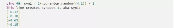
5.创建突触(即权重):行 47-48
因为输入x.shape=[4, 3],所以syn0.shape=[3, 4]
l1 = x * syn0 = [4, 3] * [3, 4] = [4, 4]
因为最后结果是四个人的答案所以l2.shape = [4, 1]
l2 = l1 * syn1 = [4, 4] * syn1 = [4, 1]
所以syn1.shape = [4, 1]
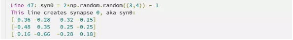
也许你会疑惑,代码行 47 中的「2」和「-1」是哪儿来的。np.random.random 函数生成均匀分布于 0 到 1 之间的随机数(对应的平均值为 0.5),而我们想让随机数初始值的平均值为 0。这样该矩阵中的初始权重不会存在偏向于 1 或 0 的先验偏置(在最开始的时候,网络不知道接下来会发生什么,因此它对其预测结果是没有信心的,直到我们在每个迭代后更新它)。
那么,我们如何将一组平均值为 0.5 的数字转变为平均值为 0 的数字呢?首先,将所有随机数乘 2(这样所有数字分布在 0 到 2 之间,平均值为 1),然后减去 1(这样所有数字分布在-1 到 1 之间,平均值为 0)。这就是「2」和「-1」出现的原因。
6.前馈网络
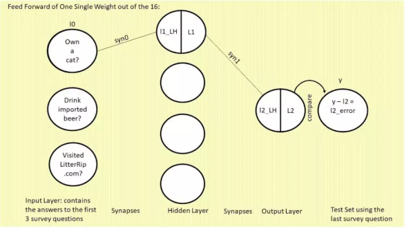
从上面第一张图中我们可以看出,syn0是4*4=16个权重,syn1是4*1=4个权重,我们以syn0,syn1中的第一个第一个权重为例,详细介绍关于前向传播的原理。
为什么表示 l2 和 l1 神经元的圆圈被从中间分割开了?圆圈的左半边(带有 LH 字样)是 sigmoid 函数的输入值,右半边是 sigmoid 函数的输出:l1 或 l2。在这个语境下,sigmoid函数只是将前一层与前一个权重相乘,并转换为 0 到 1 之间的值。代码如下
return 1/(1+np.exp(-x))
那么现在列一下用到的数值:
l0 = [1, 0, 1] (即第一个人对三个问题的回到),第一个数值为 1
syn0 = [ 3.66 -2.88 3.26 -1.53] 第一个权重为 3.66
[-4.84 3.54 2.52 -2.55]
[ 0.16 -0.66 -2.82 1.87]
为什么这个syn0与初始的syn0不同呢?假设网络已经迭代运算多次了,所以它的值会在每次迭代中更新。
现在,我们用 l0 的第一个值 1 与 syn0 的第一个值 3.66 相乘,看看会得到什么:

其运算原理如下:
l0 * syn0 = l1_LH ------> (1 * 3.66) + (0 * -4.84) + (1 * 0.16) = 3.82
sigmoid(l1_LH) = l1 ------> 1/(1+np.exp(-x)) = 1/(1+(e^-3.82)) = 0.98
l1 * syn1_1 = l2_LH ------> (0.98 * 12.1) + 【 (l1_2 * sy1_2) + (l1_2 * sy1_2) + (l1_2 * sy1_2) + (l1_2 * sy1_2) = -11.97 】 = 0.00
sigmoid(l2_LH) = l2 ------> 1/(1+np.exp(-x)) = 1/(1+(e^0)) = 0.5
y - l2 = l2_error ------> 1 - 0.5 = 0.5
上述具体解释了某一个值的运算过程,那么真实的运算如下:
l0(4, 3) * syn0(3, 4) = l1_LH(4, 4)
nonlin(l1_LH) = l1(4, 4)
l1(4, 4) * syn1(4, 1) = l2_LH(4, 1)
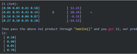
nonlin(l2_LH) = l2(4, 1)
最后的L2也就是我们的预测结果(0 ~ 1)之间的概率。代码行58,59
以上就是一次前向传播的整个计算过程
7.利用梯度下降调整网络参数
「梯度」就是「坡度」,「梯度下降」即计算某一点到最优点的最优坡度。
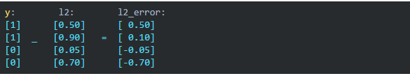
7.1 梯度下降的第一步即,计算当前的预测结果与真值 y(1/yes 或 0/no)之间的差距。
代码66行(计算误差)
l2_error = y - l2

'''
y = [
    [1],
    [1],
    [0],
    [0]
]

l2 = [
    [ 0.50]
    [ 0.90]
    [ 0.05]
    [ 0.70]
]
'''
7.2 打印误差值 代码行 72-73
if (j% 10000)==0:
  print("Avg l2_error after 10,000 more iterations: "+str(np.mean(np.abs(l2_error))))
np.mean(np.abs(l2_error))) 取误差的绝对值,然后求平均数并打印出来,从而简化了打印过程。
现在我们已经知道预测结果(l2)距离真值(y)的距离,并打印了出来。但是,我们距离真值还是太远,我们要如何降低目前令人失望的预测误差 0.5,最终近似真值呢?很显然只能通过调整权重syn0,syn1来改变误差!
7.3 代码行 88
l2_delta = l2_error*nonlin(l2,deriv=True)
上述代码的意思是,损失值 * 预测值的坡度 = 下一次预测值的变化
再来看一下nonlin()函数。
8 def nonlin(x,deriv=False):
9   if(deriv==True):
10    return x*(1-x)
11
12  return 1/(1+np.exp(-x))
x * (1 - x) 就得出了其坡度。很多人会问为什么,如果看了上面贴的关于sigmoid函数的链接就会知道,sigmoid函数的导数便是f(x)*(1 - f(x))
如下图所示,我们可以看到l2中的值在下图描绘的点,以l2其中一个点0.9(也就是绿色点)为例。
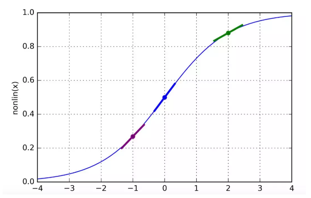
我们可以看到,越接近于1或0的值(也就是准确率高的值)其坡度越小!反之越大。我们在改变网络权重的时候往往不想改变那些使预测结果接近真值的权重,只想改变那些误差比较大的权重。事实上,这些权重的改变是由原数值乘以特别小的数字(坡度)来进行的,那么原值乘以坡度小的变化就小有用的从而有用的权重得以保留,乘以坡度大的变化就大权重得以改变。这恰好符合我们的期望。
7.4 现在我们来可视化代码88行,看一看到底是如何计算变化的
l2_delta:                       l2_error:                l2 slopes after nonlin():
[ 0.125] Big change             [ 0.50] Big Miss         [0.25] Not Confident
[ 0.009] Small-ish Change   =   [ 0.10] Small Miss    *  [0.09] Fairly Confident
[-0.003] Tiny change            [-0.05] Tiny miss        [0.05] Confident
[-0.150] Huge Change            [-0.70] Very Big Miss    [0.21] Not Confident
通过上面的等式不难看出大误差对应大坡度,大的误差(即l2_error中大的值) * 大的坡度(即通过nonlin计算得出的值) = 变化也大(即l2_delta中大的值)
l2_delta实际上就是下一次迭代中我们希望看到的 l2 的变化。
7.5 计算l1_error 代码 100 行
100 l1_error = l2_delta.dot(syn1.T)
现在我们知道下一次迭代中 l2 预测要做的改变是 l2_delta,也知道到达目前预测结果的 syn1 值。那么重要的问题来了:如果我们用 l2_delta 乘以这次迭代的 syn1 值会怎么样?这就像好莱坞编剧一样:你写了一个悲伤结局的电影,主角被龙喷出的火焰灼伤然后被吃掉,所以未能到达城堡。导演看了剧本满屋咆哮:「我要 happy ending,我要主角打败恶龙,发现生命的意义,然后转身离开!」你同意按老板的意思修改剧本。你知道了要达到的结局,就转回去寻找哪个动作出了错。哪个情节使得你没有成为英雄反而被龙吃掉?数学就是在做这样的事情:如果你把 l2_delta(期望的完美结局)乘以 syn1(导致错误结局的情节),那么你将收获 l1_error。改变造成错误结局的情节,下一版剧本将变得更好。
7.6 计算下一次l1的变化l1_delta 代码 109 行
109 l1_delta = l1_error * nonlin(l1,deriv=True)
知道了 l1_error,你就可以计算在下次迭代中将 l1 改变多少才能得到更好的 l2 预测,而这就是 l1_delta。
7.7 更新权重 代码 115 - 116 行
更新权重的数学方法即 用 (当前每一层输出 * 下一层的变化) + 上一层的权重 = 新的上一层权重
115  syn1 += l1.T.dot(l2_delta)
116  syn0 += l0.T.dot(l1_delta)
源码:
import numpy as np

def nonlin(x, deriv=False):
    if(deriv):
        return x*(1-x)
    return 1/(1+np.exp(-x))

x = np.array([
    [1, 0, 1],
    [0, 1, 1],
    [0, 0, 1],
    [1, 1, 1]
])
y = np.array([
    [1],
    [1],
    [0],
    [0]
])
np.random.seed(1)
l0 = x
syn0 = 2*np.random.rand(3, 4) - 1
syn1 = 2*np.random.rand(4, 1) - 1

for i in range(60000):
    l1 = nonlin(np.dot(l0, syn0)) #4, 4
    l2 = nonlin(np.dot(l1, syn1)) #4, 1
    l2_error = y - l2
    if (i % 10000) == 0:
        print("Avg l2_error after {} more iterations: {}".format(i, str(np.mean(np.abs(l2_error)))))
    l2_delta = l2_error * nonlin(l2, deriv=True) #4, 1 # 得到变化
    l1_error = np.dot(l2_delta, syn1.T) #4, 4
    l1_delta = l1_error*nonlin(l1, deriv=True) #4, 4 变化 = 坡度 = 每个点的导数
    syn1 += l1.T.dot(l2_delta)
    syn0 += l0.T.dot(l1_delta)

print(y)
print(l2)
打印结果:

用tensorflow来实现这一过程
import tensorflow as tf
import numpy as np

X = np.array([
    [1, 0, 1],
    [0, 1, 1],
    [0, 0, 1],
    [1, 1, 1]
])
Y = np.array([
    [1],
    [1],
    [0],
    [0]
])
np.random.seed(1)
BATCH_SIZE = 4
LR = 0.00001

#定义输入和权重
x = tf.placeholder(tf.float32, shape=(None, 3))
y_ = tf.placeholder(tf.float32, shape=(None, 1))
w1 = tf.Variable(tf.random_normal([3, 4], stddev=1, seed=1))
w2 = tf.Variable(tf.random_normal([4, 1], stddev=1, seed=1))
#定义前向传播过程
a = tf.matmul(x, w1)
y = tf.matmul(a, w2)
#定义损失函数及反向传播方法
loss = tf.reduce_mean(tf.square(y - y_))
train_step = tf.train.GradientDescentOptimizer(LR).minimize(loss)

with tf.Session() as sess:
    init = tf.global_variables_initializer()
    sess.run(init)
    setps = 6000 * 10
    for i in range(setps):
        start = (i * BATCH_SIZE) % 4
        end = start + BATCH_SIZE
        sess.run(train_step, feed_dict={x: X[start: end], y_: Y[start: end]})
        if i % 1000 == 0:
            print(sess.run(loss, feed_dict={x: X, y_: Y}))
    print(sess.run(w1))
    print(sess.run(w2))

原文链接https://colab.research.google.com/drive/1VdwQq8JJsonfT4SV0pfXKZ1vsoNvvxcH