机器学习笔记

sklearn API:http://scikit-learn.org/stable/modules/classes.html#module-sklearn.model_selection

GaussianNB

有关地形数据的GaussianNB 部署:

#!/usr/bin/python

""" Complete the code in ClassifyNB.py with the sklearn
    Naive Bayes classifier to classify the terrain data.
    
    The objective of this exercise is to recreate the decision 
    boundary found in the lesson video, and make a plot that
    visually shows the decision boundary """


from prep_terrain_data import makeTerrainData
from class_vis import prettyPicture, output_image
from ClassifyNB import classify
from sklearn.naive_bayes import GaussianNB
import numpy as np
import pylab as pl


features_train, labels_train, features_test, labels_test = makeTerrainData()

### the training data (features_train, labels_train) have both "fast" and "slow" points mixed
### in together--separate them so we can give them different colors in the scatterplot,
### and visually identify them
grade_fast = [features_train[ii][0] for ii in range(0, len(features_train)) if labels_train[ii]==0]
bumpy_fast = [features_train[ii][1] for ii in range(0, len(features_train)) if labels_train[ii]==0]
grade_slow = [features_train[ii][0] for ii in range(0, len(features_train)) if labels_train[ii]==1]
bumpy_slow = [features_train[ii][1] for ii in range(0, len(features_train)) if labels_train[ii]==1]

# You will need to complete this function imported from the ClassifyNB script.
# Be sure to change to that code tab to complete this quiz.
clf = classify(features_train, labels_train)

### draw the decision boundary with the text points overlaid
prettyPicture(clf, features_test, labels_test)
output_image("test.png", "png", open("test.png", "rb").read())

#!/usr/bin/python

#from udacityplots import *
import warnings
warnings.filterwarnings("ignore")

import matplotlib 
matplotlib.use('agg')

import matplotlib.pyplot as plt
import pylab as pl
import numpy as np

#import numpy as np
#import matplotlib.pyplot as plt
#plt.ioff()

def prettyPicture(clf, X_test, y_test):
    x_min = 0.0; x_max = 1.0
    y_min = 0.0; y_max = 1.0

    # Plot the decision boundary. For that, we will assign a color to each
    # point in the mesh [x_min, m_max]x[y_min, y_max].
    h = .01  # step size in the mesh
    xx, yy = np.meshgrid(np.arange(x_min, x_max, h), np.arange(y_min, y_max, h))
    Z = clf.predict(np.c_[xx.ravel(), yy.ravel()])

    # Put the result into a color plot
    Z = Z.reshape(xx.shape)
    plt.xlim(xx.min(), xx.max())
    plt.ylim(yy.min(), yy.max())

    plt.pcolormesh(xx, yy, Z, cmap=pl.cm.seismic)

    # Plot also the test points
    grade_sig = [X_test[ii][0] for ii in range(0, len(X_test)) if y_test[ii]==0]
    bumpy_sig = [X_test[ii][1] for ii in range(0, len(X_test)) if y_test[ii]==0]
    grade_bkg = [X_test[ii][0] for ii in range(0, len(X_test)) if y_test[ii]==1]
    bumpy_bkg = [X_test[ii][1] for ii in range(0, len(X_test)) if y_test[ii]==1]

    plt.scatter(grade_sig, bumpy_sig, color = "b", label="fast")
    plt.scatter(grade_bkg, bumpy_bkg, color = "r", label="slow")
    plt.legend()
    plt.xlabel("bumpiness")
    plt.ylabel("grade")

    plt.savefig("test.png")
    
import base64
import json
import subprocess

def output_image(name, format, bytes):
    image_start = "BEGIN_IMAGE_f9825uweof8jw9fj4r8"
    image_end = "END_IMAGE_0238jfw08fjsiufhw8frs"
    data = {}
    data['name'] = name
    data['format'] = format
    data['bytes'] = base64.encodestring(bytes)
    print image_start+json.dumps(data)+image_end

#!/usr/bin/python
import random


def makeTerrainData(n_points=1000):
###############################################################################
### make the toy dataset
    random.seed(42)
    grade = [random.random() for ii in range(0,n_points)]
    bumpy = [random.random() for ii in range(0,n_points)]
    error = [random.random() for ii in range(0,n_points)]
    y = [round(grade[ii]*bumpy[ii]+0.3+0.1*error[ii]) for ii in range(0,n_points)]
    for ii in range(0, len(y)):
        if grade[ii]>0.8 or bumpy[ii]>0.8:
            y[ii] = 1.0

### split into train/test sets
    X = [[gg, ss] for gg, ss in zip(grade, bumpy)]
    split = int(0.75*n_points)
    X_train = X[0:split]
    X_test  = X[split:]
    y_train = y[0:split]
    y_test  = y[split:]

    grade_sig = [X_train[ii][0] for ii in range(0, len(X_train)) if y_train[ii]==0]
    bumpy_sig = [X_train[ii][1] for ii in range(0, len(X_train)) if y_train[ii]==0]
    grade_bkg = [X_train[ii][0] for ii in range(0, len(X_train)) if y_train[ii]==1]
    bumpy_bkg = [X_train[ii][1] for ii in range(0, len(X_train)) if y_train[ii]==1]

#    training_data = {"fast":{"grade":grade_sig, "bumpiness":bumpy_sig}
#            , "slow":{"grade":grade_bkg, "bumpiness":bumpy_bkg}}


    grade_sig = [X_test[ii][0] for ii in range(0, len(X_test)) if y_test[ii]==0]
    bumpy_sig = [X_test[ii][1] for ii in range(0, len(X_test)) if y_test[ii]==0]
    grade_bkg = [X_test[ii][0] for ii in range(0, len(X_test)) if y_test[ii]==1]
    bumpy_bkg = [X_test[ii][1] for ii in range(0, len(X_test)) if y_test[ii]==1]

    test_data = {"fast":{"grade":grade_sig, "bumpiness":bumpy_sig}
            , "slow":{"grade":grade_bkg, "bumpiness":bumpy_bkg}}

    return X_train, y_train, X_test, y_test
#    return training_data, test_data

from sklearn.naive_bayes import GaussianNB
def classify(features_train, labels_train):   
    ### import the sklearn module for GaussianNB
    ### create classifier
    ### fit the classifier on the training features and labels
    ### return the fit classifier
    
    
    ### your code goes here!
    
    clf=GaussianNB()
    clf.fit(features_train,labels_train)
   
    return clf.fit(features_train,labels_train)

计算 GaussianNB 准确性:

def NBAccuracy(features_train, labels_train, features_test, labels_test):
    """ compute the accuracy of your Naive Bayes classifier """
    ### import the sklearn module for GaussianNB
    from sklearn.naive_bayes import GaussianNB

    ### create classifier
    clf = GaussianNB()

    ### fit the classifier on the training features and labels
    #TODO
    clf.fit(features_train,labels_train)
    ### use the trained classifier to predict labels for the test features
    pred = clf.predict(features_test)


    ### calculate and return the accuracy on the test data
    ### this is slightly different than the example, 
    ### where we just print the accuracy
    ### you might need to import an sklearn module
    from sklearn.metrics import accuracy_score
 #   print accuracy_score(pred,labels_test)
    accuracy =accuracy_score(pred,labels_test)
    return accuracy

from class_vis import prettyPicture
from prep_terrain_data import makeTerrainData
from classify import NBAccuracy

import matplotlib.pyplot as plt
import numpy as np
import pylab as pl


features_train, labels_train, features_test, labels_test = makeTerrainData()

def submitAccuracy():
    accuracy = NBAccuracy(features_train, labels_train, features_test, labels_test)
    return accuracy

支持向量机（sport vertor）

1、使用参考资料：http://scikit-learn.org/stable/modules/svm.html

2、支持向量机相关代码：

import sys
from class_vis import prettyPicture
from prep_terrain_data import makeTerrainData

import matplotlib.pyplot as plt
import copy
import numpy as np
import pylab as pl


features_train, labels_train, features_test, labels_test = makeTerrainData()


########################## SVM #################################
### we handle the import statement and SVC creation for you here
from sklearn.svm import SVC
clf = SVC(kernel="linear")


#### now your job is to fit the classifier
#### using the training features/labels, and to
#### make a set of predictions on the test data
clf.fit(features_train,labels_train)


#### store your predictions in a list named pred

pred=clf.predict(features_test)



from sklearn.metrics import accuracy_score
acc = accuracy_score(pred, labels_test)

def submitAccuracy():
    return acc

 决策树（decision tree）

1、参考资料：http://scikit-learn.org/stable/modules/tree.html

                      http://www.jianshu.com/p/c2916d616acc

2、相关代码：

#!/usr/bin/python

""" lecture and example code for decision tree unit """

import sys
from class_vis import prettyPicture, output_image
from prep_terrain_data import makeTerrainData

import matplotlib.pyplot as plt
import numpy as np
import pylab as pl
from classifyDT import classify

features_train, labels_train, features_test, labels_test = makeTerrainData()

### the classify() function in classifyDT is where the magic
### happens--fill in this function in the file 'classifyDT.py'!
clf = classify(features_train, labels_train)


#### grader code, do not modify below this line

prettyPicture(clf, features_test, labels_test)
output_image("test.png", "png", open("test.png", "rb").read())

复制代码

def classify(features_train, labels_train):
    
    ### your code goes here--should return a trained decision tree classifer
    from sklearn import tree
    clf=tree.DecisionTreeRegressor()
    pred=clf.fit(features_train,labels_train)
    return pred

决策树的准确性：

import sys
from class_vis import prettyPicture
from prep_terrain_data import makeTerrainData

import numpy as np
import pylab as pl

features_train, labels_train, features_test, labels_test = makeTerrainData()



#################################################################################


########################## DECISION TREE #################################



#### your code goes here
from sklearn import tree
clf=tree.DecisionTreeRegressor()
clf.fit(features_train,labels_train)
pred=clf.predict(features_test)

from sklearn.metrics import accuracy_score
acc = accuracy_score(pred, labels_test)

#acc = ### you fill this in!
### be sure to compute the accuracy on the test set


    
def submitAccuracies():
  return {"acc":round(acc,3)}

决策树参数:

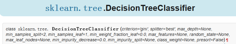
 通过使用决策树参数min_samples_split=2,min_samples_split=50比较决策树的准确性

import sys
from class_vis import prettyPicture
from prep_terrain_data import makeTerrainData

import matplotlib.pyplot as plt
import numpy as np
import pylab as pl

features_train, labels_train, features_test, labels_test = makeTerrainData()

########################## DECISION TREE #################################
### your code goes here--now create 2 decision tree classifiers,
### one with min_samples_split=2 and one with min_samples_split=50
### compute the accuracies on the testing data and store
### the accuracy numbers to acc_min_samples_split_2 and
### acc_min_samples_split_50, respectively

from sklearn import tree
clf_2=tree.DecisionTreeClassifier(min_samples_split=2)
clf_2.fit(features_train,labels_train)
pred_2=clf_2.predict(features_test)

clf_50=tree.DecisionTreeClassifier(min_samples_split=50)
clf_50.fit(features_train,labels_train)
pred_50=clf_50.predict(features_test)

from sklearn.metrics import accuracy_score
acc_min_samples_split_2=accuracy_score(pred_2,labels_test)
acc_min_samples_split_50=accuracy_score(pred_50,labels_test)

from sklearn.tree import DecisionTreeClassifier
def submitAccuracies():
  return {"acc_min_samples_split_2":round(acc_min_samples_split_2,3),
          "acc_min_samples_split_50":round(acc_min_samples_split_50,3)}

运行结果：

{"message": "{'acc_min_samples_split_50': 0.912, 'acc_min_samples_split_2': 0.908}"}

熵、条件熵、信息增益：

参考：https://www.zhihu.com/question/22104055

熵：表示随机变量的不确定性。

条件熵：在一个条件下，随机变量的不确定性。

信息增益：熵 - 条件熵

线性回归（linearRegression）

1、搜索sklearn regression 可找到相关资料

2、参考资料：http://scikit-learn.org/stable/modules/generated/sklearn.linear_model.LinearRegression.html

3、相关代码：

年龄/净值回归代码

#!/usr/bin/python

import numpy
import matplotlib
matplotlib.use('agg')

import matplotlib.pyplot as plt
from studentRegression import studentReg
from class_vis import prettyPicture, output_image

from ages_net_worths import ageNetWorthData

ages_train, ages_test, net_worths_train, net_worths_test = ageNetWorthData()

reg = studentReg(ages_train, net_worths_train)

plt.clf()
plt.scatter(ages_train, net_worths_train, color="b", label="train data")
plt.scatter(ages_test, net_worths_test, color="r", label="test data")
plt.plot(ages_test, reg.predict(ages_test), color="black")
plt.legend(loc=2)
plt.xlabel("ages")
plt.ylabel("net worths")

plt.savefig("test.png")
output_image("test.png", "png", open("test.png", "rb").read())

def studentReg(ages_train, net_worths_train):
    ### import the sklearn regression module, create, and train your regression
    ### name your regression reg
    
    ### your code goes here!
    from sklearn.linear_model import LinearRegression
    clf=LinearRegression()
    reg=clf.fit(ages_train,net_worths_train)
    
    return reg

reg.coef_  :斜率

reg.intercept:截距

reg.score:

在sklearn 中训练/测试分离

参考：http://scikit-learn.org/stable/modules/cross_validation.html

X_train, X_test, y_train, y_test = train_test_split(
...     iris.data, iris.target, test_size=0.4, random_state=0)

相关代码：

#!/usr/bin/python

""" 
PLEASE NOTE:
The api of train_test_split changed and moved from sklearn.cross_validation to
sklearn.model_selection(version update from 0.17 to 0.18)

The correct documentation for this quiz is here: 
http://scikit-learn.org/0.17/modules/cross_validation.html
"""

from sklearn import datasets
from sklearn.svm import SVC

iris = datasets.load_iris()
features = iris.data
labels = iris.target

###############################################################
### YOUR CODE HERE
###############################################################

### import the relevant code and make your train/test split
### name the output datasets features_train, features_test,
### labels_train, and labels_test
# PLEASE NOTE: The import here changes depending on your version of sklearn
from sklearn import cross_validation # for version 0.17
# For version 0.18
# from sklearn.model_selection import train_test_split

### set the random_state to 0 and the test_size to 0.4 so
### we can exactly check your result
features_train, features_test, labels_train, labels_test = cross_validation.train_test_split(iris.data, iris.target, test_size=0.4, random_state=0)

###############################################################
# DONT CHANGE ANYTHING HERE
clf = SVC(kernel="linear", C=1.)
clf.fit(features_train, labels_train)

print clf.score(features_test, labels_test)
##############################################################
def submitAcc():
    return clf.score(features_test, labels_test)

def submitAcc():
    return clf.score(features_test, labels_test)

结果：0.966666666667

k折交叉验证（k-fold cross validation）

 sklearn中的 GridSearchCV

GridSearchCV 用于系统地遍历多种参数组合，通过交叉验证确定最佳效果参数。它的好处是，只需增加几行代码，就能遍历多种组合。

下面是来自 sklearn 文档 的一个示例：

parameters = {'kernel':('linear', 'rbf'), 'C':[1, 10]}
svr = svm.SVC()
clf = grid_search.GridSearchCV(svr, parameters)
clf.fit(iris.data, iris.target)

让我们逐行进行说明。

parameters = {'kernel':('linear', 'rbf'), 'C':[1, 10]}

参数字典以及他们可取的值。在这种情况下，他们在尝试找到 kernel（可能的选择为 'linear' 和 'rbf' ）和 C（可能的选择为1和10）的最佳组合。

这时，会自动生成一个不同（kernel、C）参数值组成的“网格”:

('rbf', 1)	('rbf', 10)
('linear', 1)	('linear', 10)

各组合均用于训练 SVM，并使用交叉验证对表现进行评估。

svr = svm.SVC() 
这与创建分类器有点类似，就如我们从第一节课一直在做的一样。但是请注意，“clf” 到下一行才会生成—这儿仅仅是在说采用哪种算法。另一种思考方法是，“分类器”在这种情况下不仅仅是一个算法，而是算法加参数值。请注意，这里不需对 kernel 或 C 做各种尝试；下一行才处理这个问题。

clf = grid_search.GridSearchCV(svr, parameters) 
这是第一个不可思议之处，分类器创建好了。 我们传达算法 (svr) 和参数 (parameters) 字典来尝试，它生成一个网格的参数组合进行尝试。

clf.fit(iris.data, iris.target) 
第二个不可思议之处。 拟合函数现在尝试了所有的参数组合，并返回一个合适的分类器，自动调整至最佳参数组合。现在您便可通过 clf.best_params_ 来获得参数值。

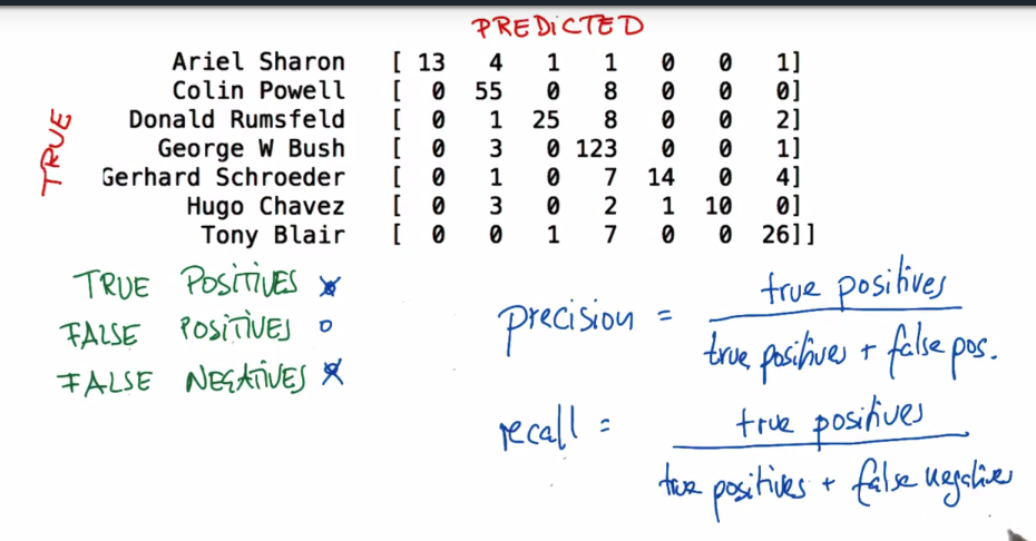
精确率（prcision）与召回率（recall）

以Colin Powell为例子

true positive （真正例）：把Colin Powell预测成Colin Powell（55）

false positive（假正例）：把其他人预测成Colin Powell（4+1+3+1+3）

false negative（假负例）：把Colin Powell预测成其他人（8）

F1 分数

既然我们已讨论了精确率和召回率，接下来可能要考虑的另一个指标是 F1 分数。F1 分数会同时考虑精确率和召回率，以便计算新的分数。

可将 F1 分数理解为精确率和召回率的加权平均值，其中 F1 分数的最佳值为 1、最差值为 0：

F1 = 2 * (精确率 * 召回率) / (精确率 + 召回率)

有关 F1 分数和如何在 sklearn 中使用它的更多信息，请查看此链接此处。

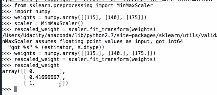
特征缩放

http://scikit-learn.org/stable/modules/preprocessing.html