支持向量机系列
(1) 算法理论理解
http://blog.pluskid.org/?page_id=683
手把手教你实现SVM算法(一)
(2) 算法应用
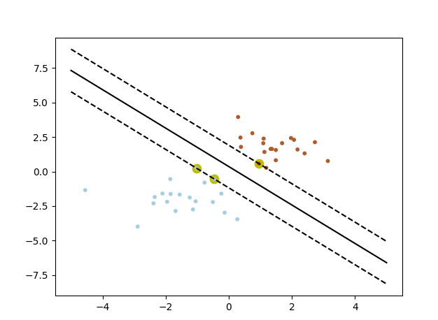
算法应用----python 实现实例,线性分割二维平面数据
工具: python 以及numpy matplot sklearn
sklearn的svm的介绍以及一些实例
http://scikit-learn.org/stable/modules/generated/sklearn.svm.SVC.html
# coding: utf-8
#1 sklearn简单例子

from sklearn import svm

X = [[2, 0], [1, 1], [2,3]]
y = [0, 0, 1]
clf = svm.SVC(kernel = 'linear')
clf.fit(X, y)

print(clf)

# get support vectors
print(clf.support_vectors_)

# get indices of support vectors
print(clf.support_)

# get number of support vectors for each class
print(clf.n_support_)


# coding: utf-8
#2 sklearn画出决定界限
print(__doc__)

import numpy as np
import pylab as pl
from sklearn import svm

# we create 40 separable points
np.random.seed(0)
#随机数据
X = np.r_[np.random.randn(20, 2) - [2, 2], np.random.randn(20, 2) + [2, 2]]
#数据标签
label = [0] * 20 + [1] * 20
print(label)

# fit the model
clf = svm.SVC(kernel='linear')
clf.fit(X, label)

# get the separating hyperplane
w = clf.coef_[0]
a = -w[0] / w[1]
wb = clf.intercept_[0]
print( "w: ", w)
print( "a: ", a)
print("wb: ", wb)

#超平面方程求解
# w[0] * x + w[1] * y + wb = 0
# y = (-w[0] / w[1]) * x - wb / w[1]
xx = np.linspace(-5, 5)
yy = a * xx - (clf.intercept_[0]) / w[1]

#支撑平面求解
# plot the parallels to the separating hyperplane that pass through the
# support vectors
# y = a * x + b
spoint = clf.support_vectors_[0]#获取分类为0的支持向量点
# x = spoint[0] y = spoint[1]; spoint[1] = a * spoint[0] = b
yy_down = a * xx + (spoint[1] - a * spoint[0])

spoint = clf.support_vectors_[-1]#获取分类为1的支持向量点
yy_up = a * xx + (spoint[1] - a * spoint[0])


# print( " xx: ", xx)
# print( " yy: ", yy)
print( "support_vectors_: ", clf.support_vectors_)
print( "clf.coef_: ", clf.coef_)

# In scikit-learn coef_ attribute holds the vectors of the separating hyperplanes for linear models. It has shape (n_classes, n_features) if n_classes > 1 (multi-class one-vs-all) and (1, n_features) for binary classification.
#
# In this toy binary classification example, n_features == 2, hence w = coef_[0] is the vector orthogonal to the hyperplane (the hyperplane is fully defined by it + the intercept).
#
# To plot this hyperplane in the 2D case (any hyperplane of a 2D plane is a 1D line), we want to find a f as in y = f(x) = a.x + b. In this case a is the slope of the line and can be computed by a = -w[0] / w[1].


#分割平面
# plot the line, the points, and the nearest vectors to the plane
pl.plot(xx, yy, 'k-')
pl.plot(xx, yy_down, 'k--')
pl.plot(xx, yy_up, 'k--')

#支持向量点 黄色粗笔
pl.scatter(clf.support_vectors_[:, 0], clf.support_vectors_[:, 1], s=80, c='y', cmap=pl.cm.Paired)
#数据点
pl.scatter(X[:, 0], X[:, 1], s = 10, c=label, cmap=pl.cm.Paired)

pl.axis('tight')
pl.show()
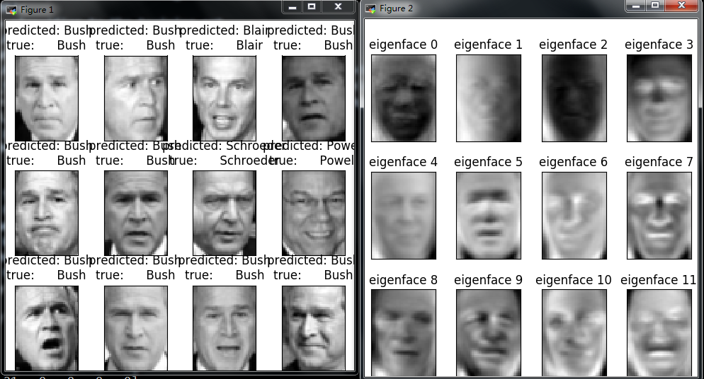
(3) 人脸识别实例
"""
===================================================
Faces recognition example using eigenfaces and SVMs
===================================================

The dataset used in this example is a preprocessed excerpt of the
"Labeled Faces in the Wild", aka LFW_:

  http://vis-www.cs.umass.edu/lfw/lfw-funneled.tgz (233MB)

.. _LFW: http://vis-www.cs.umass.edu/lfw/

Expected results for the top 5 most represented people in the dataset:

================== ============ ======= ========== =======
                   precision    recall  f1-score   support
================== ============ ======= ========== =======
     Ariel Sharon       0.67      0.92      0.77        13
     Colin Powell       0.75      0.78      0.76        60
  Donald Rumsfeld       0.78      0.67      0.72        27
    George W Bush       0.86      0.86      0.86       146
Gerhard Schroeder       0.76      0.76      0.76        25
      Hugo Chavez       0.67      0.67      0.67        15
       Tony Blair       0.81      0.69      0.75        36

      avg / total       0.80      0.80      0.80       322
================== ============ ======= ========== =======

"""
from __future__ import print_function

from time import time
import logging
import matplotlib.pyplot as plt

from sklearn.model_selection import train_test_split
from sklearn.model_selection import GridSearchCV
from sklearn.datasets import fetch_lfw_people
from sklearn.metrics import classification_report
from sklearn.metrics import confusion_matrix
from sklearn.decomposition import PCA
from sklearn.svm import SVC


print(__doc__)

# Display progress logs on stdout
logging.basicConfig(level=logging.INFO, format='%(asctime)s %(message)s')


# #############################################################################
# Download the data, if not already on disk and load it as numpy arrays

lfw_people = fetch_lfw_people(min_faces_per_person=70, resize=0.4)

# introspect the images arrays to find the shapes (for plotting)
n_samples, h, w = lfw_people.images.shape

# for machine learning we use the 2 data directly (as relative pixel
# positions info is ignored by this model)
X = lfw_people.data
n_features = X.shape[1]

# the label to predict is the id of the person
y = lfw_people.target
target_names = lfw_people.target_names
n_classes = target_names.shape[0]

print("Total dataset size:")
print("n_samples: %d" % n_samples)
print("n_features: %d" % n_features)
print("n_classes: %d" % n_classes)


# #############################################################################
# Split into a training set and a test set using a stratified k fold

# split into a training and testing set
X_train, X_test, y_train, y_test = train_test_split(
    X, y, test_size=0.25, random_state=42)


# #############################################################################
# Compute a PCA (eigenfaces) on the face dataset (treated as unlabeled
# dataset): unsupervised feature extraction / dimensionality reduction
n_components = 150

print("Extracting the top %d eigenfaces from %d faces"
      % (n_components, X_train.shape[0]))
t0 = time()
pca = PCA(n_components=n_components, svd_solver='randomized',
          whiten=True).fit(X_train)
print("done in %0.3fs" % (time() - t0))

eigenfaces = pca.components_.reshape((n_components, h, w))

print("Projecting the input data on the eigenfaces orthonormal basis")
t0 = time()
X_train_pca = pca.transform(X_train)
X_test_pca = pca.transform(X_test)
print("done in %0.3fs" % (time() - t0))


# #############################################################################
# Train a SVM classification model

print("Fitting the classifier to the training set")
t0 = time()
param_grid = {'C': [1e3, 5e3, 1e4, 5e4, 1e5],
              'gamma': [0.0001, 0.0005, 0.001, 0.005, 0.01, 0.1], }
clf = GridSearchCV(SVC(kernel='rbf', class_weight='balanced'), param_grid)
clf = clf.fit(X_train_pca, y_train)
print("done in %0.3fs" % (time() - t0))
print("Best estimator found by grid search:")
print(clf.best_estimator_)


# #############################################################################
# Quantitative evaluation of the model quality on the test set

print("Predicting people's names on the test set")
t0 = time()
y_pred = clf.predict(X_test_pca)
print("done in %0.3fs" % (time() - t0))

print(classification_report(y_test, y_pred, target_names=target_names))
print(confusion_matrix(y_test, y_pred, labels=range(n_classes)))


# #############################################################################
# Qualitative evaluation of the predictions using matplotlib

def plot_gallery(images, titles, h, w, n_row=3, n_col=4):
    """Helper function to plot a gallery of portraits"""
    plt.figure(figsize=(1.8 * n_col, 2.4 * n_row))
    plt.subplots_adjust(bottom=0, left=.01, right=.99, top=.90, hspace=.35)
    for i in range(n_row * n_col):
        plt.subplot(n_row, n_col, i + 1)
        plt.imshow(images[i].reshape((h, w)), cmap=plt.cm.gray)
        plt.title(titles[i], size=12)
        plt.xticks(())
        plt.yticks(())


# plot the result of the prediction on a portion of the test set

def title(y_pred, y_test, target_names, i):
    pred_name = target_names[y_pred[i]].rsplit(' ', 1)[-1]
    true_name = target_names[y_test[i]].rsplit(' ', 1)[-1]
    return 'predicted: %s
true:      %s' % (pred_name, true_name)

prediction_titles = [title(y_pred, y_test, target_names, i)
                     for i in range(y_pred.shape[0])]

plot_gallery(X_test, prediction_titles, h, w)

# plot the gallery of the most significative eigenfaces

eigenface_titles = ["eigenface %d" % i for i in range(eigenfaces.shape[0])]
plot_gallery(eigenfaces, eigenface_titles, h, w)

plt.show()
out
===================================================
Faces recognition example using eigenfaces and SVMs
===================================================
The dataset used in this example is a preprocessed excerpt of the
"Labeled Faces in the Wild", aka LFW_:
http://vis-www.cs.umass.edu/lfw/lfw-funneled.tgz (233MB)
.. _LFW: http://vis-www.cs.umass.edu/lfw/
Expected results for the top 5 most represented people in the dataset:
================== ============ ======= ========== =======
precision recall f1-score support
================== ============ ======= ========== =======
Ariel Sharon 0.67 0.92 0.77 13
Colin Powell 0.75 0.78 0.76 60
Donald Rumsfeld 0.78 0.67 0.72 27
George W Bush 0.86 0.86 0.86 146
Gerhard Schroeder 0.76 0.76 0.76 25
Hugo Chavez 0.67 0.67 0.67 15
Tony Blair 0.81 0.69 0.75 36
avg / total 0.80 0.80 0.80 322
================== ============ ======= ========== =======
Total dataset size:
n_samples: 1288
n_features: 1850
n_classes: 7
Extracting the top 150 eigenfaces from 966 faces
done in 0.080s
Projecting the input data on the eigenfaces orthonormal basis
done in 0.007s
Fitting the classifier to the training set
done in 22.160s
Best estimator found by grid search:
SVC(C=1000.0, cache_size=200, class_weight='balanced', coef0=0.0,
decision_function_shape='ovr', degree=3, gamma=0.001, kernel='rbf',
max_iter=-1, probability=False, random_state=None, shrinking=True,
tol=0.001, verbose=False)
Predicting people's names on the test set
done in 0.047s
precision recall f1-score support
Ariel Sharon 0.53 0.62 0.57 13
Colin Powell 0.76 0.88 0.82 60
Donald Rumsfeld 0.74 0.74 0.74 27
George W Bush 0.93 0.88 0.91 146
Gerhard Schroeder 0.80 0.80 0.80 25
Hugo Chavez 0.69 0.60 0.64 15
Tony Blair 0.88 0.81 0.84 36
avg / total 0.84 0.83 0.83 322
[[ 8 2 2 1 0 0 0]
[ 2 53 2 2 0 1 0]
[ 4 0 20 2 0 1 0]
[ 1 10 1 129 3 1 1]
[ 0 2 0 1 20 1 1]
[ 0 1 0 1 2 9 2]
[ 0 2 2 3 0 0 29]]