题目链接:http://www.spoj.com/problems/COT2/
学会了树上莫队,真的是太激动了!
参照博客:http://codeforces.com/blog/entry/43230 讲的十分清楚。(代码后面附翻译)
#include<bits/stdc++.h>
using namespace std;

const int MAXN=40005;
const int maxm=100005;

int cur;
int sat[MAXN];
int ean[MAXN];
int A[MAXN*2];
int a[MAXN];
int cou[MAXN];
int vis[MAXN];

int block_size;

struct Query
{
    int id;
    int l,r;
    int ex;
    bool operator < (const Query& q) const
    {
        int b1=(l-1)/block_size;
        int b2=(q.l-1)/block_size;
        return b1<b2 || b1==b2 && r<q.r;
    }
} query[maxm];
int ans[maxm];

int rmq[2*MAXN];//rmq数组,就是欧拉序列对应的深度序列
struct ST
{
    int mm[2*MAXN];
    int dp[2*MAXN][20];//最小值对应的下标
    void init(int n)
    {
        mm[0] = -1;
        for(int i = 1; i <= n; i++)
        {
            mm[i] = ((i&(i-1)) == 0)?mm[i-1]+1:mm[i-1];
            dp[i][0] = i;
        }
        for(int j = 1; j <= mm[n]; j++)
            for(int i = 1; i + (1<<j) - 1 <= n; i++)
                dp[i][j] = rmq[dp[i][j-1]] <
                           rmq[dp[i+(1<<(j-1))][j-1]]?dp[i][j-1]:dp[i+(1<<(j-1))][j-1];
    }
    int query(int a,int b)//查询[a,b]之间最小值的下标
    {
        if(a > b)swap(a,b);
        int k = mm[b-a+1];
        return rmq[dp[a][k]] <=
               rmq[dp[b-(1<<k)+1][k]]?dp[a][k]:dp[b-(1<<k)+1][k];
    }
};
//边的结构体定义
struct Edge
{
    int to,next;
};
Edge edge[MAXN*2];
int tot,head[MAXN];
int F[MAXN*2];//欧拉序列,就是dfs遍历的顺序,长度为2*n-1,下标从1开始
int P[MAXN];//P[i]表示点i在F中第一次出现的位置
int cnt;
ST st;
void init()
{
    tot = 0;
    memset(head,-1,sizeof(head));
}
void addedge(int u,int v)//加边,无向边需要加两次
{
    edge[tot].to = v;
    edge[tot].next = head[u];
    head[u] = tot++;
}
void dfs(int u,int pre,int dep)
{
    sat[u]=++cur;
    F[++cnt] = u;
    rmq[cnt] = dep;
    P[u] = cnt;
    for(int i = head[u]; i != -1; i = edge[i].next)
    {
        int v = edge[i].to;
        if(v == pre)continue;
        dfs(v,u,dep+1);
        F[++cnt] = u;
        rmq[cnt] = dep;
    }
    ean[u]=++cur;
}
void LCA_init(int root,int node_num)//查询LCA前的初始化
{
    cnt = 0;
    dfs(root,root,0);
    st.init(2*node_num-1);
}
int query_lca(int u,int v)//查询u,v的lca编号
{
    return F[st.query(P[u],P[v])];
}

vector<int> ls;
int nowL,nowR,nowAns;

void inc(int i)  // add or remove a[i]
{
    if (vis[i])
    {
        cou[a[i]]--;
        vis[i]^=1;
        if (cou[a[i]]==0) nowAns--;
    }
    else
    {
        cou[a[i]]++;
        vis[i]^=1;
        if (cou[a[i]]==1) nowAns++;
    }
}

int main()
{
    int n,m;
    scanf("%d%d",&n,&m);
    for (int i=1; i<=n; i++) scanf("%d",&a[i]);
    for (int i=1; i<=n; i++) ls.push_back(a[i]);
    sort(ls.begin(),ls.end());
    ls.erase(unique(ls.begin(),ls.end()),ls.end());
    for (int i=1; i<=n; i++) a[i]=lower_bound(ls.begin(),ls.end(),a[i])-ls.begin()+1;
    init();
    for(int i = 1; i < n; i++)
    {
        int u,v;
        scanf("%d%d",&u,&v);
        addedge(u,v);
        addedge(v,u);
    }
    LCA_init(1,n);
    for (int i=1; i<=n; i++) A[sat[i]]=i;
    for (int i=1; i<=n; i++) A[ean[i]]=i;
    block_size=(int)sqrt(cur)+1;
    for (int i=1; i<=m; i++)
    {
        int u,v;
        scanf("%d%d",&u,&v);
        if (sat[u]>sat[v]) swap(u,v);
        int lc=query_lca(u,v);
        if (lc==u)
        {
            query[i].l=sat[u];
            query[i].r=sat[v];
            query[i].ex=-1;
            query[i].id=i;
        }
        else
        {
            query[i].l=ean[u];
            query[i].r=sat[v];
            query[i].ex=sat[lc];
            query[i].id=i;
        }
    }
    sort(query+1,query+1+m);
    for (int i=1; i<=m; i++)
    {
        while (nowR<query[i].r)
        {
            nowR++;
            inc(A[nowR]);
        }
        while (nowL>query[i].l)
        {
            nowL--;
            inc(A[nowL]);
        }
        while (nowR>query[i].r)
        {
            inc(A[nowR]);
            nowR--;
        }
        while (nowL<query[i].l)
        {
            if (nowL) inc(A[nowL]);
            nowL++;
        }
        if (query[i].ex!=-1) inc(A[query[i].ex]);
        ans[query[i].id]=nowAns;
        if (query[i].ex!=-1) inc(A[query[i].ex]);
    }
    for (int i=1; i<=m; i++) printf("%d
",ans[i]);
    return 0;
}
由于 http://codeforces.com/blog/entry/43230 这篇博客讲的太好了,所以在这里简要翻译一下,以便以后复习。
首先,一维的莫队算法是n*sqrt(n)的复杂度。对于树形的问题,如果是子树相关的问题,想用莫队可以直接按dfs序转化成一维的。
但是有些问题不是子树的问题,但是依然可以用莫队算法,这类问题就是树上莫队问题,一般来说是处理树的路径上的性质。树上莫队掌握了基本的原理以后其实都是很套路的。
比如spoj COT2这个题就是比较经典的树上莫队,要查询的是路径上不同的数的个数。
Observation(s)
Let a node u have k children. Let us number them as v1,v2...vk. Let S(u) denote the subtree rooted at u.
Let us assume that dfs() will visit u's children in the order v1,v2...vk. Let x be any node in S(vi) and y be any node in S(vj) and let i < j. Notice that dfs(y) will be called only after dfs(x) has been completed and S(x) has been explored. Thus, before we call dfs(y), we would have entered and exited S(x). We will exploit this seemingly obvious property of dfs() to modify our existing algorithm and try to represent each query as a contiguous range in a flattened array.
观察
假设u有k个孩子,分别是v1,v2,...,vk。设S(u)表示以u为根的子树。
假定dfs()函数会按照v1,v2,...,vk的顺序遍历u的孩子。设i<j,那么设x是S(vi)中的任意一个节点,y是S(vj)中的任意一个节点。注意到dfs(y)一定在dfs(x)完成之后调用。所以在我们调用dfs(y)之前,我们一定已经遍历完了S(x)。我们会用这个看似显然的dfs性质,来对我们已经知道的处理子树的莫队算法稍作修改,就可以把处理的路径变成一段一维上的连续区间。
Modified DFS-Order
Let us modify the dfs order as follows. For each node u, maintain the Start and End time of S(u). Let's call them ST(u) and EN(u). The only change you need to make is that you must increment the global timekeeping variable even when you finish traversing some subtree (EN(u) = ++cur). In short, we will maintain 2 values for each node u. One will denote the time when you entered S(u) and the other would denote the time when you exited S(u).Consider the tree in the picture. Given below are the ST() and EN() values of the nodes.
修改后的dfs序
对dfs序做如下修改。对于每一个节点u,维护S(u)的开始和结束时间戳,设为ST(u)和EN(u)。与一般的dfs不同的是,不仅要ST(u)=++cur,还要有EN(u)=++cur。可以看下面这个图片的例子,并且给出了每个节点的ST和EN。以及每个时间戳的访问情况。
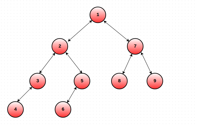
ST(1) = 1 EN(1) = 18
ST(2) = 2 EN(2) = 11
ST(3) = 3 EN(3) = 6
ST(4) = 4 EN(4) = 5
ST(5) = 7 EN(5) = 10
ST(6) = 8 EN(6) = 9
ST(7) = 12 EN(7) = 17
ST(8) = 13 EN(8) = 14
ST(9) = 15 EN(9) = 16
A[] = {1, 2, 3, 4, 4, 3, 5, 6, 6, 5, 2, 7, 8, 8, 9, 9, 7, 1}
The Algorithm
Now that we're equipped with the necessary weapons, let's understand how to process the queries.
Let a query be (u, v). We will try to map each query to a range in the flattened array. Let ST(u) ≤ ST(v) where ST(u) denotes visit time of node u in T. Let P = LCA(u, v) denote the lowest common ancestor of nodes u and v. There are 2 possible cases:
算法
现在,我们已经掌握了必要的工具,让我们理解一下怎么处理路径上的查询吧。
假设查询是(u,v)。我们会尽力把每一个查询都映射到一段一维区间上。(之所以说尽力,是因为有时候会多出一个单点)
不妨设ST(u)<=ST(v),设P是u和v的lca(最近公共祖先lca算法http://www.cnblogs.com/acmsong/p/7543507.html),有两种可能的情况。
Case 1: P = u
In this case, our query range would be [ST(u), ST(v)]. Why will this work?
Consider any node x that does not lie in the (u, v) path.
Notice that x occurs twice or zero times in our specified query range.
Therefore, the nodes which occur exactly once in this range are precisely those that are on the (u, v) path! (Try to convince yourself of why this is true : It's all because of dfs()properties.)
This forms the crux of our algorithm. While implementing Mo's, our add/remove function needs to check the number of times a particular node appears in a range. If it occurs twice (or zero times), then we don't take it's value into account! This can be easily implemented while moving the left and right pointers.
情况1:P=u
在这种情况下,我们的查询就是在[ST(u), ST(v)]内出现奇数次的数字。(译者注:这里说的区间是时间戳区间,类似于上面的这个A[] = {1, 2, 3, 4, 4, 3, 5, 6, 6, 5, 2, 7, 8, 8, 9, 9, 7, 1},而出现奇数次还是偶数次,这个问题本身就是用一维莫队就能维护的,当一个数字变成奇数次以后,就加上它的影响,当一个数字变成偶数次的时候,就减去它的影响。)为什么这个区间是对的呢?
设不在u到v路径上的任意一点为x,注意到x在我们给定的这段区间里要么出现2次,要么出现0次,而u到v路径上的点都只出现了1次,相信吧:都是因为dfs序的性质!(这里也没给证明。。。)
Case 2: P ≠ u
In this case, our query range would be [EN(u), ST(v)] + [ST(P), ST(P)].
The same logic as Case 1 applies here as well. The only difference is that we need to consider the value of P i.e the LCA separately, as it would not be counted in the query range.
情况2:P≠u
在这种情况下,我们的查询区间是[EN(u), ST(v)] + [ST(P), ST(P)]。基本逻辑与情况1是相同的,只不过多出来一个单点要单独考虑。
至此,这个算法就结束了。