注:因为公式敲起来太麻烦,因此本文中的公式没有呈现出来,想要知道具体的计算公式,请参考原书中内容
降维就是指采用某种映射方法,将原高维空间中的数据点映射到低维度的空间中
1、主成分分析(PCA)
将n维样本X通过投影矩阵W,转换为K维矩阵Z
输入:样本集D,低维空间d
输出:投影矩阵W
算法步骤:
1)对所有样本进行中心化操作
2)计算样本的协方差矩阵
3)对协方差矩阵做特征值分解
4)取最大的d个特征值对应的特征向量,构造投影矩阵W
注:通常低维空间维数d的选取有两种方法:1)通过交叉验证法选取较好的d 2)从算法原理的角度设置一个阈值,比如t=0.95,然后选取似的下式成立的最小的d值:
Σ(i->d)λi/Σ(i->n)λi>=t,其中λi从大到小排列
PCA降维的准则有以下两个:
最近重构性:重构后的点距离原来的点的误差之和最小
最大可分性:样本点在低维空间的投影尽可能分开
实验代码:


 1 import numpy as np
 2 import matplotlib.pyplot as plt
 3 from sklearn import datasets,decomposition,manifold
 4
 5 def load_data():
 6     iris=datasets.load_iris()
 7     return iris.data,iris.target
 8
 9 def test_PCA(*data):
10     X,Y=data
11     pca=decomposition.PCA(n_components=None)
12     pca.fit(X)
13     print("explained variance ratio:%s"%str(pca.explained_variance_ratio_))
14
15 def plot_PCA(*data):
16     X,Y=data
17     pca=decomposition.PCA(n_components=2)
18     pca.fit(X)
19     X_r=pca.transform(X)
20  #   print(X_r)
21
22     fig=plt.figure()
23     ax=fig.add_subplot(1,1,1)
24     colors=((1,0,0),(0,1,0),(0,0,1),(0.5,0.5,0),(0,0.5,0.5),(0.5,0,0.5),(0.4,0.6,0),(0.6,0.4,0),(0,0.6,0.4),(0.5,0.3,0.2),)
25     for label,color in zip(np.unique(Y),colors):
26         position=Y==label
27   #      print(position)
28         ax.scatter(X_r[position,0],X_r[position,1],label="target=%d"%label,color=color)
29     ax.set_xlabel("X[0]")
30     ax.set_ylabel("Y[0]")
31     ax.legend(loc="best")
32     ax.set_title("PCA")
33     plt.show()
34
35 X,Y=load_data()
36 test_PCA(X,Y)
37 plot_PCA(X,Y)
实验结果:
可以看出四个特征值的比例分别占比0.92464621,0.05301557,0.01718514,0.00518309,因此可将原始特征4维降低到2维

IncrementalPCA超大规模数据降维
可以使用与超大规模数据,它可以将数据分批加载进内存,其接口和用法几乎与PCA完全一致
2、SVD降维
SVD奇异值分解等价于PCA主成分分析,核心都是求解X*(X转置)的特征值以及对应的特征向量
3、核化线性(KPCA)降维
是一种非线性映射的方法,核主成分分析是对PCA的一种推广
实验代码:
import numpy as np
import matplotlib.pyplot as plt
from sklearn import datasets,decomposition,manifold

def load_data():
    iris=datasets.load_iris()
    return iris.data,iris.target

def test_KPCA(*data):
    X,Y=data
    kernels=['linear','poly','rbf','sigmoid']
    for kernel in kernels:
        kpca=decomposition.KernelPCA(n_components=None,kernel=kernel)
        kpca.fit(X)
        print("kernel=%s-->lambdas:%s"%(kernel,kpca.lambdas_))

def plot_KPCA(*data):
    X,Y=data
    kernels = ['linear', 'poly', 'rbf', 'sigmoid']
    fig=plt.figure()
    colors=((1,0,0),(0,1,0),(0,0,1),(0.5,0.5,0),(0,0.5,0.5),(0.5,0,0.5),(0.4,0.6,0),(0.6,0.4,0),(0,0.6,0.4),(0.5,0.3,0.2),)
    for i,kernel in enumerate(kernels):
        kpca=decomposition.KernelPCA(n_components=2,kernel=kernel)
        kpca.fit(X)
        X_r=kpca.transform(X)
        ax=fig.add_subplot(2,2,i+1)
        for label,color in zip(np.unique(Y),colors):
            position=Y==label
            ax.scatter(X_r[position,0],X_r[position,1],label="target=%d"%label,color=color)
            ax.set_xlabel("X[0]")
            ax.set_ylabel("X[1]")
            ax.legend(loc="best")
            ax.set_title("kernel=%s"%kernel)
    plt.suptitle("KPCA")
    plt.show()


X,Y=load_data()
test_KPCA(X,Y)
plot_KPCA(X,Y)
实验结果:
不同的核函数,其降维后的数据分布是不同的
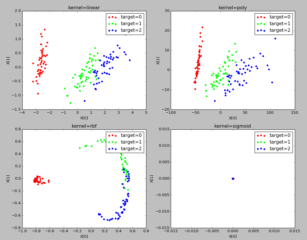
并且采用同样的多项式核函数,如果参数不同,其降维后的数据分布是不同的。因此再具体应用中,可以通过选用不同的核函数以及设置多种不同的参数来对比哪种情况下可以获得最好的效果。
4、流形学习降维
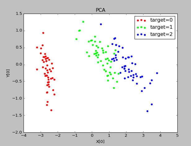
是一种借鉴了拓扑流形概念的降维方法
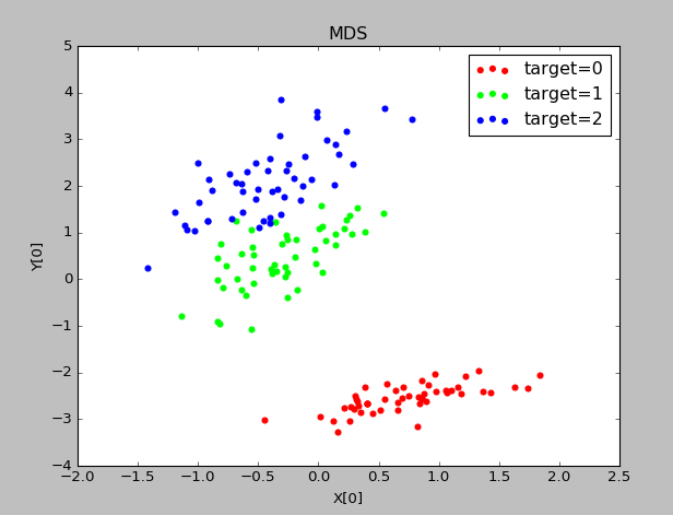
5、多维缩放(MDS)降维
MDS要求原始空间中样本之间的距离在低维空间中得到保持
输入:距离矩阵D,低维空间维数n'
输出:样本集在低维空间中的矩阵Z
算法步骤:
1)依据公式计算di,.^2,dj,.^2,d.,.^2
2)依据公式计算降维后空间的内积矩阵B
3)对矩阵B进行特征值分解
4)依据求得的对角矩阵和特征向量矩阵,依据公式计算Z
实验代码:
import numpy as np
import matplotlib.pyplot as plt
from sklearn import datasets,decomposition,manifold

def load_data():
    iris=datasets.load_iris()
    return iris.data,iris.target

def test_MDS(*data):
    X,Y=data
    for n in [4,3,2,1]:
        mds=manifold.MDS(n_components=n)
        mds.fit(X)
        print("stress(n_components=%d):%s"%(n,str(mds.stress_)))

def plot_MDS(*data):
    X,Y=data
    mds=manifold.MDS(n_components=2)
    X_r=mds.fit_transform(X)
 #   print(X_r)

    fig=plt.figure()
    ax=fig.add_subplot(1,1,1)
    colors=((1,0,0),(0,1,0),(0,0,1),(0.5,0.5,0),(0,0.5,0.5),(0.5,0,0.5),(0.4,0.6,0),(0.6,0.4,0),(0,0.6,0.4),(0.5,0.3,0.2),)
    for label,color in zip(np.unique(Y),colors):
        position=Y==label
        ax.scatter(X_r[position,0],X_r[position,1],label="target=%d"%label,color=color)
    ax.set_xlabel("X[0]")
    ax.set_ylabel("Y[0]")
    ax.legend(loc="best")
    ax.set_title("MDS")
    plt.show()

X,Y=load_data()
test_MDS(X,Y)
plot_MDS(X,Y)
实验结果:
stress表示原始数据降维后的距离误差之和

6、等度量映射(Isomap)降维
输入:样本集D,近邻参数k,低维空间维数n’
输出:样本集在低维空间中的矩阵Z
算法步骤:
1)对每个样本点x,计算它的k近邻;同时将x与它的k近邻的距离设置为欧氏距离,与其他点的距离设置为无穷大
2)调用最短路径算法计算任意两个样本点之间的距离,获得距离矩阵D
3)调用多维缩放MDS算法,获得样本集在低维空间中的矩阵Z
注:新样本难以将其映射到低维空间中,因此需要训练一个回归学习器来对新样本的低维空间进行预测
建立近邻图时,要控制好距离的阈值,防止短路和断路
实验代码:
 1 import numpy as np
 2 import matplotlib.pyplot as plt
 3 from sklearn import datasets,decomposition,manifold
 4
 5 def load_data():
 6     iris=datasets.load_iris()
 7     return iris.data,iris.target
 8
 9 def test_Isomap(*data):
10     X,Y=data
11     for n in [4,3,2,1]:
12         isomap=manifold.Isomap(n_components=n)
13         isomap.fit(X)
14         print("reconstruction_error(n_components=%d):%s"%(n,isomap.reconstruction_error()))
15
16 def plot_Isomap_k(*data):
17     X,Y=data
18     Ks=[1,5,25,Y.size-1]
19     fig=plt.figure()
20   #  colors=((1,0,0),(0,1,0),(0,0,1),(0.5,0.5,0),(0,0.5,0.5),(0.5,0,0.5),(0.4,0.6,0),(0.6,0.4,0),(0,0.6,0.4),(0.5,0.3,0.2),)
21     for i,k in enumerate(Ks):
22         isomap=manifold.Isomap(n_components=2,n_neighbors=k)
23         X_r=isomap.fit_transform(X)
24         ax=fig.add_subplot(2,2,i+1)
25         colors = ((1, 0, 0), (0, 1, 0), (0, 0, 1), (0.5, 0.5, 0), (0, 0.5, 0.5), (0.5, 0, 0.5), (0.4, 0.6, 0), (0.6, 0.4, 0),
26         (0, 0.6, 0.4), (0.5, 0.3, 0.2),)
27         for label,color in zip(np.unique(Y),colors):
28             position=Y==label
29             ax.scatter(X_r[position,0],X_r[position,1],label="target=%d"%label,color=color)
30     ax.set_xlabel("X[0]")
31     ax.set_ylabel("Y[0]")
32     ax.legend(loc="best")
33     ax.set_title("k=%d"%k)
34     plt.suptitle("Isomap")
35     plt.show()
36
37 X,Y=load_data()
38 test_Isomap(X,Y)
39 plot_Isomap_k(X,Y)
实验结果:

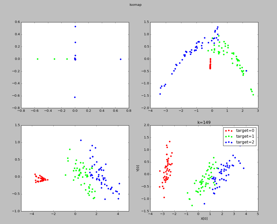
可以看出k=1时,近邻范围过小,此时发生断路现象
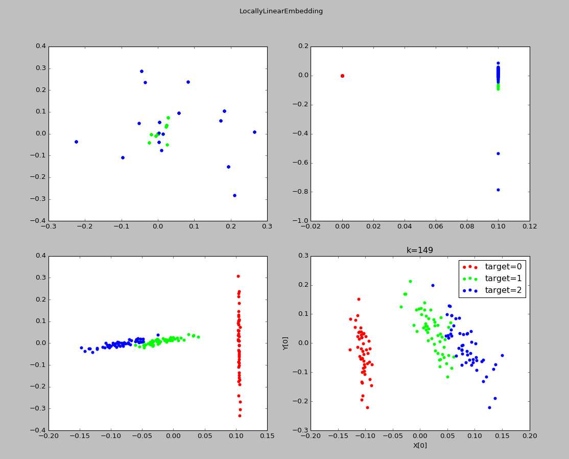
7、局部线性嵌入(LLE)
其目标是保持邻域内样本之间的线性关系
输入:样本集D,近邻参数k,低维空间维数n'
输出:样本集在低维空间中的矩阵Z
算法步骤:
1)对于样本集中的每个点x,确定其k近邻,获得其近邻下标集合Q,然后依据公式计算Wi,j
2)根据Wi,j构建矩阵W
3)依据公式计算M
4)对M进行特征值分解,取其最小的n'个特征值对应的特征向量,即得到样本集在低维空间中的矩阵Z
实验代码:
 1 import numpy as np
 2 import matplotlib.pyplot as plt
 3 from sklearn import datasets,decomposition,manifold
 4
 5 def load_data():
 6     iris=datasets.load_iris()
 7     return iris.data,iris.target
 8
 9 def test_LocallyLinearEmbedding(*data):
10     X,Y=data
11     for n in [4,3,2,1]:
12         lle=manifold.LocallyLinearEmbedding(n_components=n)
13         lle.fit(X)
14         print("reconstruction_error_(n_components=%d):%s"%(n,lle.reconstruction_error_))
15
16 def plot_LocallyLinearEmbedding_k(*data):
17     X,Y=data
18     Ks=[1,5,25,Y.size-1]
19     fig=plt.figure()
20   #  colors=((1,0,0),(0,1,0),(0,0,1),(0.5,0.5,0),(0,0.5,0.5),(0.5,0,0.5),(0.4,0.6,0),(0.6,0.4,0),(0,0.6,0.4),(0.5,0.3,0.2),)
21     for i,k in enumerate(Ks):
22         lle=manifold.LocallyLinearEmbedding(n_components=2,n_neighbors=k)
23         X_r=lle.fit_transform(X)
24         ax=fig.add_subplot(2,2,i+1)
25         colors = ((1, 0, 0), (0, 1, 0), (0, 0, 1), (0.5, 0.5, 0), (0, 0.5, 0.5), (0.5, 0, 0.5), (0.4, 0.6, 0), (0.6, 0.4, 0),
26         (0, 0.6, 0.4), (0.5, 0.3, 0.2),)
27         for label,color in zip(np.unique(Y),colors):
28             position=Y==label
29             ax.scatter(X_r[position,0],X_r[position,1],label="target=%d"%label,color=color)
30     ax.set_xlabel("X[0]")
31     ax.set_ylabel("Y[0]")
32     ax.legend(loc="best")
33     ax.set_title("k=%d"%k)
34     plt.suptitle("LocallyLinearEmbedding")
35     plt.show()
36
37 X,Y=load_data()
38 test_LocallyLinearEmbedding(X,Y)
39 plot_LocallyLinearEmbedding_k(X,Y)
实验结果:

8、总结:
对原始数据采取降维的原因通常有两个:缓解“维度灾难”或者对数据进行可视化。
降维的好坏没有一个直接的标准(包括上面提到的重构误差也只能作为一个中性的指标)。通常通过对数据进行降维,然后用降维后的数据进行学习,再根据学习的效果选择一个恰当的降维方式和一个合适的降维模型参数。