作者信息关联
5.1 任务说明
- 学习主题:作者关联(数据建模任务),对论文作者关系进行建模,统计最常出现的作者关系;
- 学习内容:构建作者关系图,挖掘作者关系
- 学习成果:论文作者知识图谱、图关系挖掘
5.2 数据处理步骤
将作者列表进行处理,并完成统计。具体步骤如下:
- 将论文第一作者与其他作者(论文非第一作者)构建图
- 使用图算法统计图中作者与其他作者的联系
5.3 社交网络分析
图是复杂⽹网络研究中的⼀一个重要概念。 Graph是用点和线来刻画离散事物集合中的每对事物间以某种方式相联系的数学模型。Graph在现实世界中随处可见,如交通运输图、旅游图、流程图等。利用图可以描述现实生活中的许多事物,如用点可以表示交叉口,点之间的连线表示路径,这样就可以轻而易举地描绘出⼀个交通运输网络。
5.3.1 图类型
- 无向图,忽略了两节点间边地方向
- 有向图,考虑了边的有向性
- 多重无向图,即两个节点之间的边数多余一条,又允许顶点之间通过同一条边和自己关联
5.3.2 图统计指标
- 度:是指和该节点相关联的边的条数,又称关联度。对于有向图,节点的入度 是指进入该节点的边的条数;节点的出度是指从该节点出发的边的条数;
- 迪杰斯特拉路径: 从⼀一个源点到其它各点的最短路径,可使用迪杰斯特拉算法来求最短路径;
- 连通图:在⼀个无向图G中,若从顶点i到顶点j有路径相连,则称i和j是连通的。如果 G 是有向图,那么连接i和j的路径中所有的边都必须同向。如果图中任意两点都是连通的,那么图被称作连通图。如果此图是有向图,则称为强连通图。
对于其他图算法,可以在networkx和igraph两个库中找到。
代码
import seaborn as sns
from bs4 import BeautifulSoup
import re
import requests
import json
import pandas as pd
import matplotlib.pyplot as plt
from tqdm import tqdm
import networkx as nx
from ast import literal_eval
#读取数据
data=pd.read_csv("data.csv")
D:anaconda3libsite-packagesIPythoncoreinteractiveshell.py:3146: DtypeWarning: Columns (0) have mixed types.Specify dtype option on import or set low_memory=False.
  has_raised = await self.run_ast_nodes(code_ast.body, cell_name,
data=data['authors_parsed']
data=pd.DataFrame(data)
data.head()
| authors_parsed | |
|---|---|
| 0 | [['Balázs', 'C.', ''], ['Berger', 'E. L.', '']... |
| 1 | [['Streinu', 'Ileana', ''], ['Theran', 'Louis'... |
| 2 | [['Pan', 'Hongjun', '']] |
| 3 | [['Callan', 'David', '']] |
| 4 | [['Abu-Shammala', 'Wael', ''], ['Torchinsky', ... |
# 创建⽆无向图
G = nx.Graph()

# 用十篇论⽂文进行构建
for row in data.iloc[:10].itertuples():
    authors=literal_eval(row[1])
    authors= [' '.join(x[:-1]) for x in authors]
    print(authors)

    #将第一个作者与其他作者相连
    for author in authors[1:]:
        G.add_edge(authors[0],author)
['Balázs C.', 'Berger E. L.', 'Nadolsky P. M.', 'Yuan C. -P.']
['Streinu Ileana', 'Theran Louis']
['Pan Hongjun']
['Callan David']
['Abu-Shammala Wael', 'Torchinsky Alberto']
['Pong Y. H.', 'Law C. K.']
['Corichi Alejandro', 'Vukasinac Tatjana', 'Zapata Jose A.']
['Swift Damian C.']
['Harvey Paul', 'Merin Bruno', 'Huard Tracy L.', 'Rebull Luisa M.', 'Chapman Nicholas', 'Evans Neal J.', 'Myers Philip C.']
['Ovchinnikov Sergei']
literal_eval将该形式的字符串转为list
关于itertuples,参考:https://pandas.pydata.org/pandas-docs/stable/reference/api/pandas.DataFrame.itertuples.html
#作者关系图
nx.draw(G,with_labels=True)
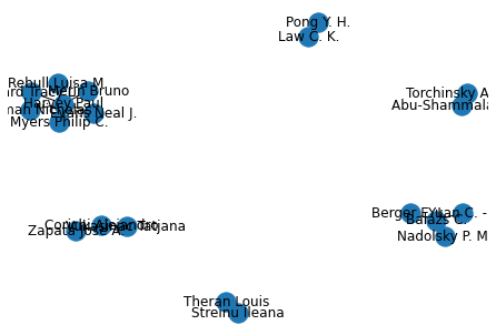
十篇论文中,六位论文有一位以上作者,四篇论文为单一作者
# 计算作者之间的距离
def distance(author1,author2):
    try:
        ans=nx.dijkstra_path(G,author1,author2)
    except:
        ans='No path'
    return ans


print(distance('Corichi Alejandro','Zapata Jose A.'))
print(distance('Corichi Alejandro','Streinu Ileana'))
['Corichi Alejandro', 'Zapata Jose A.']
No path
#以500篇论文构建,得到更完整的作者关系
G500 = nx.Graph()
for row in data.iloc[2000:2500].itertuples():
    authors=literal_eval(row[1])
    authors= [' '.join(x[:-1]) for x in authors]
    for author in authors[1:]:
        G500.add_edge(authors[0],author)
'Corichi Alejandro' in G500.nodes()
False
nx.draw(G500)

# 计算论⽂文关系中有多少个联通子图
# print(len(nx.communicability(G500)))
degree_sequence = [d for n, d in G500.degree()]
degree_sequence.sort(reverse=True)
degree_sequence
[56,
 35,
 25,
 25,
 21,
 20,
 20,
 18,
 18,
 12,
 12,
 12,
 11,
 10,
 10,
 10,
 10,
 9,
 8,
 8,
 8,
 7,
 7,
 7,
 7,
 7,
 7,
 6,
 6,
 6,
 6,
 6,
 6,
 6,
 6,
 6,
 6,
 6,
 6,
 5,
 5,
 5,
 5,
 5,
 5,
 5,
 5,
 5,
 5,
 5,
 5,
 5,
 5,
 5,
 5,
 5,
 5,
 5,
 5,
 5,
 5,
 5,
 5,
 4,
 4,
 4,
 4,
 4,
 4,
 4,
 4,
 4,
 4,
 4,
 4,
 4,
 4,
 4,
 4,
 4,
 4,
 4,
 4,
 4,
 4,
 4,
 3,
 3,
 3,
 3,
 3,
 3,
 3,
 3,
 3,
 3,
 3,
 3,
 3,
 3,
 3,
 3,
 3,
 3,
 3,
 3,
 3,
 3,
 3,
 3,
 3,
 3,
 3,
 3,
 3,
 3,
 3,
 3,
 3,
 3,
 3,
 3,
 3,
 3,
 3,
 3,
 3,
 3,
 3,
 3,
 3,
 3,
 3,
 3,
 3,
 3,
 3,
 2,
 2,
 2,
 2,
 2,
 2,
 2,
 2,
 2,
 2,
 2,
 2,
 2,
 2,
 2,
 2,
 2,
 2,
 2,
 2,
 2,
 2,
 2,
 2,
 2,
 2,
 2,
 2,
 2,
 2,
 2,
 2,
 2,
 2,
 2,
 2,
 2,
 2,
 2,
 2,
 2,
 2,
 2,
 2,
 2,
 2,
 2,
 2,
 2,
 2,
 2,
 2,
 2,
 2,
 2,
 2,
 2,
 2,
 2,
 2,
 2,
 2,
 2,
 2,
 2,
 2,
 2,
 2,
 2,
 2,
 2,
 2,
 2,
 2,
 2,
 2,
 2,
 2,
 2,
 2,
 2,
 2,
 2,
 2,
 2,
 2,
 2,
 2,
 2,
 2,
 2,
 2,
 2,
 2,
 2,
 2,
 2,
 2,
 2,
 2,
 2,
 2,
 2,
 2,
 2,
 2,
 2,
 2,
 2,
 2,
 2,
 2,
 2,
 2,
 2,
 2,
 2,
 2,
 2,
 2,
 2,
 2,
 2,
 1,
 1,
 1,
 1,
 1,
 1,
 1,
 1,
 1,
 1,
 1,
 1,
 1,
 1,
 1,
 1,
 1,
 1,
 1,
 1,
 1,
 1,
 1,
 1,
 1,
 1,
 1,
 1,
 1,
 1,
 1,
 1,
 1,
 1,
 1,
 1,
 1,
 1,
 1,
 1,
 1,
 1,
 1,
 1,
 1,
 1,
 1,
 1,
 1,
 1,
 1,
 1,
 1,
 1,
 1,
 1,
 1,
 1,
 1,
 1,
 1,
 1,
 1,
 1,
 1,
 1,
 1,
 1,
 1,
 1,
 1,
 1,
 1,
 1,
 1,
 1,
 1,
 1,
 1,
 1,
 1,
 1,
 1,
 1,
 1,
 1,
 1,
 1,
 1,
 1,
 1,
 1,
 1,
 1,
 1,
 1,
 1,
 1,
 1,
 1,
 1,
 1,
 1,
 1,
 1,
 1,
 1,
 1,
 1,
 1,
 1,
 1,
 1,
 1,
 1,
 1,
 1,
 1,
 1,
 1,
 1,
 1,
 1,
 1,
 1,
 1,
 1,
 1,
 1,
 1,
 1,
 1,
 1,
 1,
 1,
 1,
 1,
 1,
 1,
 1,
 1,
 1,
 1,
 1,
 1,
 1,
 1,
 1,
 1,
 1,
 1,
 1,
 1,
 1,
 1,
 1,
 1,
 1,
 1,
 1,
 1,
 1,
 1,
 1,
 1,
 1,
 1,
 1,
 1,
 1,
 1,
 1,
 1,
 1,
 1,
 1,
 1,
 1,
 1,
 1,
 1,
 1,
 1,
 1,
 1,
 1,
 1,
 1,
 1,
 1,
 1,
 1,
 1,
 1,
 1,
 1,
 1,
 1,
 1,
 1,
 1,
 1,
 1,
 1,
 1,
 1,
 1,
 1,
 1,
 1,
 1,
 1,
 1,
 1,
 1,
 1,
 1,
 1,
 1,
 1,
 1,
 1,
 1,
 1,
 1,
 1,
 1,
 1,
 1,
 1,
 1,
 1,
 1,
 1,
 1,
 1,
 1,
 1,
 1,
 1,
 1,
 1,
 1,
 1,
 1,
 1,
 1,
 1,
 1,
 1,
 1,
 1,
 1,
 1,
 1,
 1,
 1,
 1,
 1,
 1,
 1,
 1,
 1,
 1,
 1,
 1,
 1,
 1,
 1,
 1,
 1,
 1,
 1,
 1,
 1,
 1,
 1,
 1,
 1,
 1,
 1,
 1,
 1,
 1,
 1,
 1,
 1,
 1,
 1,
 1,
 1,
 1,
 1,
 1,
 1,
 1,
 1,
 1,
 1,
 1,
 1,
 1,
 1,
 1,
 1,
 1,
 1,
 1,
 1,
 1,
 1,
 1,
 1,
 1,
 1,
 1,
 1,
 1,
 1,
 1,
 1,
 1,
 1,
 1,
 1,
 1,
 1,
 1,
 1,
 1,
 1,
 1,
 1,
 1,
 1,
 1,
 1,
 1,
 1,
 1,
 1,
 1,
 1,
 1,
 1,
 1,
 1,
 1,
 1,
 1,
 1,
 1,
 1,
 1,
 1,
 1,
 1,
 1,
 1,
 1,
 1,
 1,
 1,
 1,
 1,
 1,
 1,
 1,
 1,
 1,
 1,
 1,
 1,
 1,
 1,
 1,
 1,
 1,
 1,
 1,
 1,
 1,
 1,
 1,
 1,
 1,
 1,
 1,
 1,
 1,
 1,
 1,
 1,
 1,
 1,
 1,
 1,
 1,
 1,
 1,
 1,
 1,
 1,
 1,
 1,
 1,
 1,
 1,
 1,
 1,
 1,
 1,
 1,
 1,
 1,
 1,
 1,
 1,
 1,
 1,
 1,
 1,
 1,
 1,
 1,
 1,
 1,
 1,
 1,
 1,
 1,
 1,
 1,
 1,
 1,
 1,
 1,
 1,
 1,
 1,
 1,
 1,
 1,
 1,
 1,
 1,
 1,
 1,
 1,
 1,
 1,
 1,
 1,
 1,
 1,
 1,
 1,
 1,
 1,
 1,
 1,
 1,
 1,
 1,
 1,
 1,
 1,
 1,
 1,
 1,
 1,
 1,
 1,
 1,
 1,
 1,
 1,
 1,
 1,
 1,
 1,
 1,
 1,
 1,
 1,
 1,
 1,
 1,
 1,
 1,
 1,
 1,
 1,
 1,
 1,
 1,
 1,
 1,
 1,
 1,
 1,
 1,
 1,
 1,
 1,
 1,
 1,
 1,
 1,
 1,
 1,
 1,
 1,
 1,
 1,
 1,
 1,
 1,
 1,
 1,
 1,
 1,
 1,
 1,
 1,
 1,
 1,
 1,
 1,
 1,
 1,
 1,
 1,
 1,
 1,
 1,
 1,
 1,
 1,
 1,
 1,
 1,
 1,
 1,
 1,
 1,
 1,
 1,
 1,
 1,
 1,
 1,
 1,
 1,
 1,
 1,
 1,
 1,
 1,
 1,
 1,
 1,
 1,
 1,
 1,
 1,
 1,
 1,
 1,
 1,
 1,
 1,
 1,
 1,
 1,
 1,
 1,
 1,
 1,
 1,
 1,
 1,
 1,
 1,
 1,
 1,
 1,
 1,
 1,
 1,
 1,
 1,
 1,
 1,
 1,
 1,
 1,
 1,
 1,
 1,
 1,
 1,
 1,
 1,
 1,
 1,
 1,
 1,
 1,
 1,
 1,
 1,
 1,
 1,
 1,
 1,
 1,
 1,
 1,
 1,
 1,
 1,
 1,
 1,
 1,
 1,
 1,
 1,
 1,
 1,
 1,
 1,
 1,
 1,
 1,
 1,
 1,
 1,
 1,
 1,
 1,
 1,
 1,
 1,
 1,
 1,
 1,
 1,
 1,
 1,
 1,
 1,
 1,
 1,
 1,
 1,
 1,
 1,
 1,
 1,
 1,
 1,
 1,
 1,
 1,
 1,
 1,
 1,
 1,
 1,
 1,
 1,
 1,
 1,
 1,
 1,
 1,
 1,
 1,
 1,
 1,
 1,
 1,
 1,
 1,
 1,
 1,
 1,
 1,
 1,
 1,
 1,
 1,
 1,
 1,
 1,
 1,
 1,
 1,
 1,
 1,
 1,
 1,
 1,
 1,
 1,
 1,
 1,
 1,
 1,
 1,
 1,
 1,
 1,
 1,
 1,
 1,
 1,
 1,
 1,
 1,
 1,
 1,
 1,
 1,
 1,
 1,
 1,
 1,
 1,
 1,
 1,
 1,
 1,
 1,
 1,
 1,
 1,
 1,
 1,
 ...]
330
关于degree_sequence,参考:https://networkx.org/documentation/stable/auto_examples/graph/plot_degree_sequence.html
plt.loglog(degree_sequence, "b-", marker="o")
plt.title("Degree rank plot")
plt.ylabel("degree")
plt.xlabel("rank")
Text(0.5, 0, 'rank')

关于plt.loglog(),参考:https://matplotlib.org/3.1.1/api/_as_gen/matplotlib.pyplot.loglog.html
# draw graph in inset
plt.axes([0.45, 0.45, 0.45, 0.45])
Gcc = G500.subgraph(sorted(nx.connected_components(G500), key=len, reverse=True)[0])#选择最大连通图
pos = nx.spring_layout(Gcc)#选择最大连通图对应的结点
plt.axis("off")
nx.draw_networkx_nodes(Gcc, pos, node_size=20)#画点
nx.draw_networkx_edges(Gcc, pos, alpha=0.4)#画边
plt.show()

plt.loglog(degree_sequence, "b-", marker="o")
plt.title("Degree rank plot")
plt.ylabel("degree")
plt.xlabel("rank")
# draw graph in inset
plt.axes([0.45, 0.45, 0.45, 0.45])
Gcc = G500.subgraph(sorted(nx.connected_components(G500), key=len, reverse=True)[0])#选择最大连通图
pos = nx.spring_layout(Gcc)#选择最大连通图对应的结点
plt.axis("off")
nx.draw_networkx_nodes(Gcc, pos, node_size=20)#画点
nx.draw_networkx_edges(Gcc, pos, alpha=0.4)#画边
plt.show()
