数据分析
概念
把隐藏在一些看似杂论无章的数据背后的信息提炼出来,总结出所研究对象的内在规律。
数据分析三剑客:Numpy、Pandas、Matplotlib
Numpy(Numerical Python)是Python语言的一个扩展程序库,支持大量的维度数组与矩阵运算,此外也针对数组运算提供大量的数学函数库。
创建ndarray
import numpy as np
使用np.array()创建
一维数据创建
np.array([1, 2, 3, 4, 5])

# 输出:
    array([1, 2, 3, 4, 5])
二维数据创建
np.array([[1, 2, 3], [4, 5, 6], [7, 8, 9]])

# 输出:
    array([[1, 2, 3],
           [4, 5, 6],
           [7, 8, 9]])
注意:
Numpy默认ndarray的所有元素的类型是相同的;
如果传进来的列表中包含不同的类型,则统一位同一类型,优先级:str > float > int;
np.array([[1, 2, 3], [4, '5', 6], [7, 8, 9]])

# 输出:
    array([['1', '2', '3'],
          ['4', '5', '6'],
          ['7', '8', '9']], dtype='<U11')
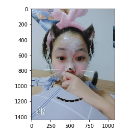
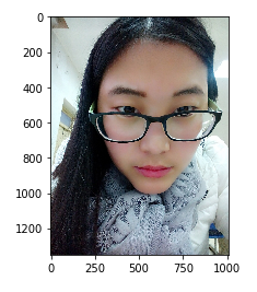
使用matplotlib.pyplot获取一个numpy数组,数据源于一张图片
import matplotlib.pyplot as plt

img_arr = plt.imread('./lmy.jpg')
plt.imshow(img_arr)

# 输出:
    <matplotlib.image.AxesImage at 0x25b81a877b8>
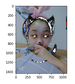
对数组进行算术运算
plt.imshow(img_arr-25)

# 输出:
    <matplotlib.image.AxesImage at 0x25b88d19080>
数组的形状
img_arr.shap

# 输出:
    (1440, 1080, 3)
操作该numpy数据,该操作会同步到图片中
使用np的routines函数创建
包含一下常见创建方法:
1) np.ones(shape, dtype=None, order='C') # 创建以1填充的指定大小的数组
np.ones(shape=(20, 30))

# 输出:
array([[1., 1., 1., 1., 1., 1., 1., 1., 1., 1., 1., 1., 1., 1., 1., 1.,
        1., 1., 1., 1., 1., 1., 1., 1., 1., 1., 1., 1., 1., 1.],
       [1., 1., 1., 1., 1., 1., 1., 1., 1., 1., 1., 1., 1., 1., 1., 1.,
        1., 1., 1., 1., 1., 1., 1., 1., 1., 1., 1., 1., 1., 1.],
       [1., 1., 1., 1., 1., 1., 1., 1., 1., 1., 1., 1., 1., 1., 1., 1.,
        1., 1., 1., 1., 1., 1., 1., 1., 1., 1., 1., 1., 1., 1.],
       [1., 1., 1., 1., 1., 1., 1., 1., 1., 1., 1., 1., 1., 1., 1., 1.,
        1., 1., 1., 1., 1., 1., 1., 1., 1., 1., 1., 1., 1., 1.],
       [1., 1., 1., 1., 1., 1., 1., 1., 1., 1., 1., 1., 1., 1., 1., 1.,
        1., 1., 1., 1., 1., 1., 1., 1., 1., 1., 1., 1., 1., 1.],
       [1., 1., 1., 1., 1., 1., 1., 1., 1., 1., 1., 1., 1., 1., 1., 1.,
        1., 1., 1., 1., 1., 1., 1., 1., 1., 1., 1., 1., 1., 1.],
       [1., 1., 1., 1., 1., 1., 1., 1., 1., 1., 1., 1., 1., 1., 1., 1.,
        1., 1., 1., 1., 1., 1., 1., 1., 1., 1., 1., 1., 1., 1.],
       [1., 1., 1., 1., 1., 1., 1., 1., 1., 1., 1., 1., 1., 1., 1., 1.,
        1., 1., 1., 1., 1., 1., 1., 1., 1., 1., 1., 1., 1., 1.],
       [1., 1., 1., 1., 1., 1., 1., 1., 1., 1., 1., 1., 1., 1., 1., 1.,
        1., 1., 1., 1., 1., 1., 1., 1., 1., 1., 1., 1., 1., 1.],
       [1., 1., 1., 1., 1., 1., 1., 1., 1., 1., 1., 1., 1., 1., 1., 1.,
        1., 1., 1., 1., 1., 1., 1., 1., 1., 1., 1., 1., 1., 1.],
       [1., 1., 1., 1., 1., 1., 1., 1., 1., 1., 1., 1., 1., 1., 1., 1.,
        1., 1., 1., 1., 1., 1., 1., 1., 1., 1., 1., 1., 1., 1.],
       [1., 1., 1., 1., 1., 1., 1., 1., 1., 1., 1., 1., 1., 1., 1., 1.,
        1., 1., 1., 1., 1., 1., 1., 1., 1., 1., 1., 1., 1., 1.],
       [1., 1., 1., 1., 1., 1., 1., 1., 1., 1., 1., 1., 1., 1., 1., 1.,
        1., 1., 1., 1., 1., 1., 1., 1., 1., 1., 1., 1., 1., 1.],
       [1., 1., 1., 1., 1., 1., 1., 1., 1., 1., 1., 1., 1., 1., 1., 1.,
        1., 1., 1., 1., 1., 1., 1., 1., 1., 1., 1., 1., 1., 1.],
       [1., 1., 1., 1., 1., 1., 1., 1., 1., 1., 1., 1., 1., 1., 1., 1.,
        1., 1., 1., 1., 1., 1., 1., 1., 1., 1., 1., 1., 1., 1.],
       [1., 1., 1., 1., 1., 1., 1., 1., 1., 1., 1., 1., 1., 1., 1., 1.,
        1., 1., 1., 1., 1., 1., 1., 1., 1., 1., 1., 1., 1., 1.],
       [1., 1., 1., 1., 1., 1., 1., 1., 1., 1., 1., 1., 1., 1., 1., 1.,
        1., 1., 1., 1., 1., 1., 1., 1., 1., 1., 1., 1., 1., 1.],
       [1., 1., 1., 1., 1., 1., 1., 1., 1., 1., 1., 1., 1., 1., 1., 1.,
        1., 1., 1., 1., 1., 1., 1., 1., 1., 1., 1., 1., 1., 1.],
       [1., 1., 1., 1., 1., 1., 1., 1., 1., 1., 1., 1., 1., 1., 1., 1.,
        1., 1., 1., 1., 1., 1., 1., 1., 1., 1., 1., 1., 1., 1.],
       [1., 1., 1., 1., 1., 1., 1., 1., 1., 1., 1., 1., 1., 1., 1., 1.,
        1., 1., 1., 1., 1., 1., 1., 1., 1., 1., 1., 1., 1., 1.]])
2) np.zeros(shape, stype=None, order='C') # 创建以1填充的指定大小的数组
np.zeros(shape=(20, 30))

# 输出:
array([[0., 0., 0., 0., 0., 0., 0., 0., 0., 0., 0., 0., 0., 0., 0., 0.,
        0., 0., 0., 0., 0., 0., 0., 0., 0., 0., 0., 0., 0., 0.],
       [0., 0., 0., 0., 0., 0., 0., 0., 0., 0., 0., 0., 0., 0., 0., 0.,
        0., 0., 0., 0., 0., 0., 0., 0., 0., 0., 0., 0., 0., 0.],
       [0., 0., 0., 0., 0., 0., 0., 0., 0., 0., 0., 0., 0., 0., 0., 0.,
        0., 0., 0., 0., 0., 0., 0., 0., 0., 0., 0., 0., 0., 0.],
       [0., 0., 0., 0., 0., 0., 0., 0., 0., 0., 0., 0., 0., 0., 0., 0.,
        0., 0., 0., 0., 0., 0., 0., 0., 0., 0., 0., 0., 0., 0.],
       [0., 0., 0., 0., 0., 0., 0., 0., 0., 0., 0., 0., 0., 0., 0., 0.,
        0., 0., 0., 0., 0., 0., 0., 0., 0., 0., 0., 0., 0., 0.],
       [0., 0., 0., 0., 0., 0., 0., 0., 0., 0., 0., 0., 0., 0., 0., 0.,
        0., 0., 0., 0., 0., 0., 0., 0., 0., 0., 0., 0., 0., 0.],
       [0., 0., 0., 0., 0., 0., 0., 0., 0., 0., 0., 0., 0., 0., 0., 0.,
        0., 0., 0., 0., 0., 0., 0., 0., 0., 0., 0., 0., 0., 0.],
       [0., 0., 0., 0., 0., 0., 0., 0., 0., 0., 0., 0., 0., 0., 0., 0.,
        0., 0., 0., 0., 0., 0., 0., 0., 0., 0., 0., 0., 0., 0.],
       [0., 0., 0., 0., 0., 0., 0., 0., 0., 0., 0., 0., 0., 0., 0., 0.,
        0., 0., 0., 0., 0., 0., 0., 0., 0., 0., 0., 0., 0., 0.],
       [0., 0., 0., 0., 0., 0., 0., 0., 0., 0., 0., 0., 0., 0., 0., 0.,
        0., 0., 0., 0., 0., 0., 0., 0., 0., 0., 0., 0., 0., 0.],
       [0., 0., 0., 0., 0., 0., 0., 0., 0., 0., 0., 0., 0., 0., 0., 0.,
        0., 0., 0., 0., 0., 0., 0., 0., 0., 0., 0., 0., 0., 0.],
       [0., 0., 0., 0., 0., 0., 0., 0., 0., 0., 0., 0., 0., 0., 0., 0.,
        0., 0., 0., 0., 0., 0., 0., 0., 0., 0., 0., 0., 0., 0.],
       [0., 0., 0., 0., 0., 0., 0., 0., 0., 0., 0., 0., 0., 0., 0., 0.,
        0., 0., 0., 0., 0., 0., 0., 0., 0., 0., 0., 0., 0., 0.],
       [0., 0., 0., 0., 0., 0., 0., 0., 0., 0., 0., 0., 0., 0., 0., 0.,
        0., 0., 0., 0., 0., 0., 0., 0., 0., 0., 0., 0., 0., 0.],
       [0., 0., 0., 0., 0., 0., 0., 0., 0., 0., 0., 0., 0., 0., 0., 0.,
        0., 0., 0., 0., 0., 0., 0., 0., 0., 0., 0., 0., 0., 0.],
       [0., 0., 0., 0., 0., 0., 0., 0., 0., 0., 0., 0., 0., 0., 0., 0.,
        0., 0., 0., 0., 0., 0., 0., 0., 0., 0., 0., 0., 0., 0.],
       [0., 0., 0., 0., 0., 0., 0., 0., 0., 0., 0., 0., 0., 0., 0., 0.,
        0., 0., 0., 0., 0., 0., 0., 0., 0., 0., 0., 0., 0., 0.],
       [0., 0., 0., 0., 0., 0., 0., 0., 0., 0., 0., 0., 0., 0., 0., 0.,
        0., 0., 0., 0., 0., 0., 0., 0., 0., 0., 0., 0., 0., 0.],
       [0., 0., 0., 0., 0., 0., 0., 0., 0., 0., 0., 0., 0., 0., 0., 0.,
        0., 0., 0., 0., 0., 0., 0., 0., 0., 0., 0., 0., 0., 0.],
       [0., 0., 0., 0., 0., 0., 0., 0., 0., 0., 0., 0., 0., 0., 0., 0.,
        0., 0., 0., 0., 0., 0., 0., 0., 0., 0., 0., 0., 0., 0.]])
3) np.full(shape, fill_value, dtype=None, order='C') # 自定义数组的大小、自定义填充的内容
np.full(shape=(5, 6), fill_value=9527)

# 输出:
array([[9527, 9527, 9527, 9527, 9527, 9527],
       [9527, 9527, 9527, 9527, 9527, 9527],
       [9527, 9527, 9527, 9527, 9527, 9527],
       [9527, 9527, 9527, 9527, 9527, 9527],
       [9527, 9527, 9527, 9527, 9527, 9527]])
4)np.linspace(start, stop, num=50, endpoint=True, restep=False, dtype=None) # 构造等差数组
np.linspace(1, 100, num=20)

# 输出:
array([  1.        ,   6.21052632,  11.42105263,  16.63157895,
        21.84210526,  27.05263158,  32.26315789,  37.47368421,
        42.68421053,  47.89473684,  53.10526316,  58.31578947,
        63.52631579,  68.73684211,  73.94736842,  79.15789474,
        84.36842105,  89.57894737,  94.78947368, 100.        ])
5)np.arange([start, ]stop, [step,]dtype-None) # 循环生成数组
np.arange(0, 100, step=2)

# 输出:
array([ 0,  2,  4,  6,  8, 10, 12, 14, 16, 18, 20, 22, 24, 26, 28, 30, 32,
       34, 36, 38, 40, 42, 44, 46, 48, 50, 52, 54, 56, 58, 60, 62, 64, 66,
       68, 70, 72, 74, 76, 78, 80, 82, 84, 86, 88, 90, 92, 94, 96, 98])
6)np.random.randint(low, high=None, size=None, dtype='l') # 随机产生指定大小的数组
np.random.randint(0, 100, size=(5, 7))

# 输出
array([[49, 10, 15, 24, 84, 64, 22],
       [39, 30, 60, 76, 53, 79,  2],
       [64, 29,  8, 89, 68,  7, 95],
       [59, 56, 86, 94, 47,  2, 18],
       [62, 72, 51, 70, 62, 34, 85]])
上边这样产生数组,每次都是不一样的,因为里边的元素都是随机产生的。
np.random.seed(5)  # 固定时间种子,产生的随机数就固定下来了
np.random.randint(0, 100, size=(5, 7))

# 输出
array([[99, 78, 61, 16, 73,  8, 62],
       [27, 30, 80,  7, 76, 15, 53],
       [80, 27, 44, 77, 75, 65, 47],
       [30, 84, 86, 18,  9, 41, 62],
       [ 1, 82, 16, 78,  5, 58,  0]])
7)np.random.randn(d0, d1, ..., dn) # 标准正太分布的数组
arr = np.random.randn(4, 5)
8) np.random.random(size=None) # 生成0到1的随机数,左闭右开
np.random.seed(3)
np.random.random(size=(3,4))

# 输出
array([[0.5507979 , 0.70814782, 0.29090474, 0.51082761],
       [0.89294695, 0.89629309, 0.12558531, 0.20724288],
       [0.0514672 , 0.44080984, 0.02987621, 0.45683322]])
ndarray的属性
4个必记参数:
ndim:维度
arr = np.random.randn(4, 5)
arr.ndim

# 输出
2
shape:形状(各维度的长度)
arr = np.random.randn(4, 5)
arr.shape

# 输出
(4, 5)
size: 总长度
arr = np.random.randn(4, 5)
arr.size

# 输出
20
dtype:元素类型
arr = np.random.randn(4, 5)
arr.dtype

# 输出
dtype('float64')
type(arr)
arr = np.random.randn(4, 5)
type(arr)

# 输出
numpy.ndarray
ndarray的基本操作
索引
一维与列表完全一致 多维时同理
arr[1][2]

# 输出
0.48624932610831123
根据索引修改数据
arr[1][2] = 1 arr # 输出 array([[-0.51664792, -0.18907167, -0.41619802, 0.72465766, -0.68996068], [ 0.48641448, 0.85151895, 1. , -0.83423985, 1.34499246], [-0.67821268, 0.42643507, -0.75333479, -1.74411025, 0.22575027], [ 0.28703516, -0.07744096, 0.2760685 , -0.64841089, -0.73746484]])
切片
一维与列表完全一致 多维时同理
arr[0: 2] # 横着切,切列;获取二维数组的前两行
arr = np.random.randint(60, 120, size=(6, 4))
arr
# arr结构
array([[ 82, 105,  96, 100],
       [ 86, 112,  69,  79],
       [100,  65, 114,  72],
       [ 86,  95,  84, 112],
       [ 94, 103, 115,  83],
       [110,  78,  60,  67]])

arr[0: 2]

# 输出
array([[ 82, 105,  96, 100],
       [ 86, 112,  69,  79]])
arr[:, 0:2] # 竖着切,切前两行;其中,左边是行,右边是列。获取二维数组的前两列。
arr[:, 0:2]

# 输出
array([[ 82, 105],
       [ 86, 112],
       [100,  65],
       [ 86,  95],
       [ 94, 103],
       [110,  78]])
获取二维数组前两行和前两列数据
arr[0: 2, 0: 2]

# 输出
array([[ 82, 105],
       [ 86, 112]])
将数据反转,例如[1, 2, 3] ---> [3, 2, 1]
:: 进行切片
将数组的行进行倒序 (将第一行换到倒数第一行,以此类推)
arr = np.random.randint(65, 130, size=(6, 4))
arr
# arr
array([[127,  91,  65, 101],
       [119, 102, 101,  88],
       [ 83, 109,  96,  76],
       [ 89,  91,  69, 121],
       [ 65,  85, 120,  75],
       [ 70, 124,  74, 119]])

arr[::-1]

# 输出
array([[ 70, 124,  74, 119],
       [ 65,  85, 120,  75],
       [ 89,  91,  69, 121],
       [ 83, 109,  96,  76],
       [119, 102, 101,  88],
       [127,  91,  65, 101]]                                                                                                                                                                                                                                                                                                                                                                                                                                                                                                                                                                                                                                                                                                        )
列倒序
arr[:, ::-1]

# 输出
array([[101,  65,  91, 127],
       [ 88, 101, 102, 119],
       [ 76,  96, 109,  83],
       [121,  69,  91,  89],
       [ 75, 120,  85,  65],
       [119,  74, 124,  70]])
全部倒序
arr[::-1, ::-1]

# 输出
array([[119,  74, 124,  70],
       [ 75, 120,  85,  65],
       [121,  69,  91,  89],
       [ 76,  96, 109,  83],
       [ 88, 101, 102, 119],
       [101,  65,  91, 127]])
将图片进行全倒置
读取图片
img_arr = plt.imread('./XiangShan.jpg')
plt.imshow(img_arr)

# 输出
<matplotlib.image.AxesImage at 0x25b88ee05c0>
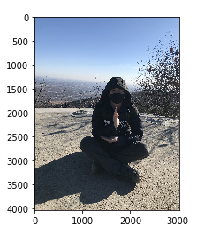
查看图片数组形状
img_arr.shape

# 输出
(4032, 3024, 3)
颜色图片倒置
plt.imshow(img_arr[:, :, ::-1])

# 输出
<matplotlib.image.AxesImage at 0x25b876810f0>

图片全倒置
plt.imshow(img_arr[::-1, ::-1, ::-1])

# 输出
<matplotlib.image.AxesImage at 0x25b876c6a58>

随机生成二维图片
my_pic_arr = np.random.randint(0,255,size=(500,500,3),dtype=np.uint8)
plt.imshow(my_pic_arr)

# 输出
<matplotlib.image.AxesImage at 0x25b890fa908>
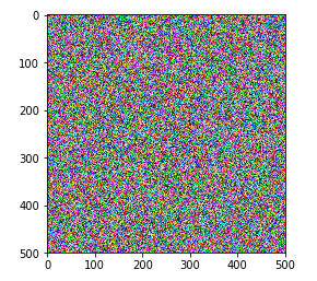
注意:
有些机器运行上述代码在没有指定dtype时,会出现 ValueError: 3-dimensional arrays must be of dtype unsigned byte, unsigned short, float32 or float64 的错误,这时只需要加上 dtype=np.uint8 就可以了,这一步操作是将编码方式指定为系统自带的编码方式。
变形
使用arr.reshape()函数,注意参数是一个tuple!
基本使用
1. 将一维数组变形成多维数组
arr

# 输出
array([[127,  91,  65, 101],
       [119, 102, 101,  88],
       [ 83, 109,  96,  76],
       [ 89,  91,  69, 121],
       [ 65,  85, 120,  75],
       [ 70, 124,  74, 119]])
arr1 = arr.reshape(24)
arr1 = arr.reshape(24)
arr1.reshape(2, 4, 3)
arr1.reshape(2, 4, 3)

# 输出
array([[[127,  91,  65],
        [101, 119, 102],
        [101,  88,  83],
        [109,  96,  76]],

       [[ 89,  91,  69],
        [121,  65,  85],
        [120,  75,  70],
        [124,  74, 119]]])
arr1.reshape(3, -1) # -1表示自动计算行数/列数
arr1.reshape(3, -1)

# 输出
array([[ 90,  73,  68, 117,  80,  65,  68,  71],
       [ 90,  83,  88, 105, 128,  97,  92, 103],
       [ 78, 105,  76,  84, 120,  98,  94,  77]])
2. 将多维数组变成一维数组
arr1 = arr.reshape(24)
arr1

# 输出
array([108, 102, 129,  76, 104, 122, 128,  88, 112, 107, 100,  87, 100,
        86,  76, 112, 110,  94,  99, 100,  90,  66, 127, 119])
图片倒置
1. 将图片读取并转化成数组
arr_img = plt.imread('./train.jpg')
2. 查看图片维度大小
arr_img.shape

# 输出
(1080, 1440, 3)
3. 将三维的图片变成一维,大小为原图片大小
arr_1_img = arr_img.reshape(1080*1440*3)
4. 对一维数组中所有的元素倒置
v_arr_1 = arr_1_img[::-1]
v_arr_1

# 输出
array([119, 119, 105, ..., 255, 255, 255], dtype=uint8)
5. 将一维数组变成三维数组
plt.imshow(v_arr_1.reshape(1080, 1440, 3))

# 输出
<matplotlib.image.AxesImage at 0x21cd33d7470>

级联
np.concatenate()
1. 一维、二维、多维数组的级联,实际操作中级联多为二维数组
生成一个6×4的数组
arr

# 输出
array([[ 90,  73,  68, 117],
       [ 80,  65,  68,  71],
       [ 90,  83,  88, 105],
       [128,  97,  92, 103],
       [ 78, 105,  76,  84],
       [120,  98,  94,  77]])
axis=0 轴向: 0表示是竖直的轴向 1表示水平的轴向
水平级联
np.concatenate((arr, arr), axis=1)

# 输出
array([[ 90,  73,  68, 117,  90,  73,  68, 117],
       [ 80,  65,  68,  71,  80,  65,  68,  71],
       [ 90,  83,  88, 105,  90,  83,  88, 105],
       [128,  97,  92, 103, 128,  97,  92, 103],
       [ 78, 105,  76,  84,  78, 105,  76,  84],
       [120,  98,  94,  77, 120,  98,  94,  77]])
竖直级联
np.concatenate((arr, arr), axis=0)

# 输出
array([[ 90,  73,  68, 117],
       [ 80,  65,  68,  71],
       [ 90,  83,  88, 105],
       [128,  97,  92, 103],
       [ 78, 105,  76,  84],
       [120,  98,  94,  77],
       [ 90,  73,  68, 117],
       [ 80,  65,  68,  71],
       [ 90,  83,  88, 105],
       [128,  97,  92, 103],
       [ 78, 105,  76,  84],
       [120,  98,  94,  77]])
准备两个数组,一个6×4, 一个3×4
arr = np.random.randint(65, 130, size=(6, 4))
arr
'''
输出
array([[ 90,  73,  68, 117],
       [ 80,  65,  68,  71],
       [ 90,  83,  88, 105],
       [128,  97,  92, 103],
       [ 78, 105,  76,  84],
       [120,  98,  94,  77]])

'''

arr1 = np.random.randint(0, 100, size=(3, 4))
arr1
'''
输出
array([[74, 62, 44, 42],
       [22, 67, 55, 10],
       [58, 26, 77, 95]])

'''
两个大小不一样的素组之间的级联
np.concatenate((arr, arr1), axis=0)
'''
输出
array([[ 90,  73,  68, 117],
       [ 80,  65,  68,  71],
       [ 90,  83,  88, 105],
       [128,  97,  92, 103],
       [ 78, 105,  76,  84],
       [120,  98,  94,  77],
       [ 74,  62,  44,  42],
       [ 22,  67,  55,  10],
       [ 58,  26,  77,  95]])
'''
一维数组无法和二维数组级联
arr1 = np.random.randint(0, 100, size=(3, 4))
arr1
'''
输出
array([[74, 62, 44, 42],
       [22, 67, 55, 10],
       [58, 26, 77, 95]])
'''

arr2 = np.array([1, 2, 3, 4])
arr2
'''
array([1, 2, 3, 4])
'''

np.concatenate((arr1, arr2), axis=0)
'''
---------------------------------------------------------------------------
ValueError                                Traceback (most recent call last)
<ipython-input-37-9b03f799ca88> in <module>()
----> 1 np.concatenate((arr1, arr2), axis=0)

ValueError: all the input arrays must have same number of dimensions
'''
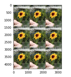
2. 合并两张照片
arr_flower = plt.imread('./flower.jpg')
arr = np.concatenate((arr_flower, arr_flower, arr_flower), axis=1)
arr_result = np.concatenate((arr, arr, arr), axis=0)
plt.imshow(arr_result)

'''
输出
<matplotlib.image.AxesImage at 0x21cd26d7208>
'''
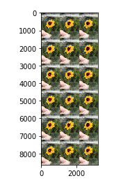
3. np.hstack与np.vstack
np.hstack
arr_flower = plt.imread('./flower.jpg')
arr = np.concatenate((arr_flower, arr_flower, arr_flower), axis=1)
arr_result = np.concatenate((arr, arr, arr), axis=0)
a = np.vstack((arr_result, arr_result))
plt.imshow(a)

'''
输出
<matplotlib.image.AxesImage at 0x21cd3474cf8>
'''
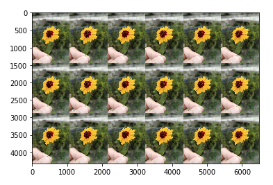
np.vstack
arr_flower = plt.imread('./flower.jpg')
arr = np.concatenate((arr_flower, arr_flower, arr_flower = plt.imread('./flower.jpg')
arr = np.concatenate((arr_flower, arr_flower, arr_flower), axis=1)
arr_result = np.concatenate((arr, arr, arr), axis=0)
a = np.vstack((arr_result, arr_result))
plt.imshow(a)arr_flower), axis=1)
arr_result = np.concatenate((arr, arr, arr), axis=0)
b = np.vstack((arr_result, arr_result))
plt.imshow(b)

'''
输出
 <matplotlib.image.AxesImage at 0x21cd30437f0>
'''
级联需要注意的点:
● 级联的参数是列表:一定要加中括号或者小括号
● 维度必须相同
● 形状相符:在维度保持一致的前提下,如果进行横向(axis=1)级联,必须保证进行级联的数组行数保持一致。如果进行纵向(axis=0)级联,必须保证进行级联的数组列数保持一致。
● 可通过axis参数改变级联的方向。
切分
与级联类似,三个函数完成切分工作:
● np.split(arr, 行/列号, 轴): 参数2是一个列表类型
● np.vsplit
● np.hsplit
获取一个数组
np.random.seed(10)
num_arr = np.random.randint(60, 100, size=(5, 6))
num_arr
'''
输出
array([[69, 96, 75, 60, 88, 85],
       [89, 89, 68, 69, 60, 96],
       [76, 96, 71, 84, 93, 68],
       [96, 74, 73, 65, 73, 85],
       [73, 88, 82, 90, 90, 85]])

'''
对数组进行分割
np.split(num_arr, [2, 3], axis=1)

'''
输出
[array([[69, 96],
        [89, 89],
        [76, 96],
        [96, 74],
        [73, 88]]), array([[75],
        [68],
        [71],
        [73],
        [82]]), array([[60, 88, 85],
        [69, 60, 96],
        [84, 93, 68],
        [65, 73, 85],
        [90, 90, 85]])]
'''
np.vsplit 切列
np.vsplit(num_arr, [2, 3])

'''
输出
[array([[69, 96, 75, 60, 88, 85],
        [89, 89, 68, 69, 60, 96]]),
 array([[76, 96, 71, 84, 93, 68]]),
 array([[96, 74, 73, 65, 73, 85],
        [73, 88, 82, 90, 90, 85]])]
'''
np.hsplit
np.hsplit(num_arr, [2, 3])

'''
输出
[array([[69, 96],
        [89, 89],
        [76, 96],
        [96, 74],
        [73, 88]]), array([[75],
        [68],
        [71],
        [73],
        [82]]), array([[60, 88, 85],
        [69, 60, 96],
        [84, 93, 68],
        [65, 73, 85],
        [90, 90, 85]])]
'''
切分照片
1. 读取照片
import matplotlib.pyplot as plt
import numpy as np

img_arr = plt.imread('./MyL.jpg')  #./MyL.jpg为图片的路径
plt.imshow(img_arr) ''' 输出 <matplotlib.image.AxesImage at 0x20d56c9a438> '''
2. 水平切
imgs = np.split(img_arr, [0, 1200], axis=0)
plt.imshow(imgs[1])

'''
输出
<matplotlib.image.AxesImage at 0x20d56f7e080>
'''
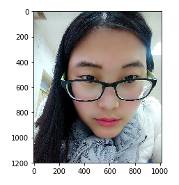
它的切割结果为三份,第一份为[0, 0], 第二份为[0, 1200],第三份为[1200, 1350]。其中,查看数组形状:
img_arr.shape

'''
输出
(1350, 1012, 3)
'''
3. 纵向切
img_data = np.split(imgs[1], [100, 1000], axis=1)[1]
plt.imshow(img_data)

'''
输出
<matplotlib.image.AxesImage at 0x20d56daf2b0>
'''
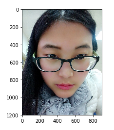
它的切割结果同样也为三份,第一份为[0, 100],第二份为[100, 1000],第三份为[1000, 1012]。
副本
所有赋值运算不会为ndarray的任何元素创建副本。对赋值后的对象的操作也对原来的对应生效。
arr = np.array([1, 2, 3, 4, 5])
a = arr.copy()
a[1] = 10

arr
'''
输出
array([1, 2, 3, 4, 5])
'''

a
'''
输出
array([ 1, 10,  3,  4,  5])
'''
ndarray的聚合操作
求和 np.sum()
a = np.array([1, 10, 3, 4, 5])
s.sum()

'''
输出
23
'''
对所有元素进行累加求和。
最大值(np.max())/最小值(np.min())
a = np.array([1, 10, 3, 4, 5])
a.max()
'''
输出
10
'''
a.min()
'''
输出
1
'''
0