随机梯度下降法的调试

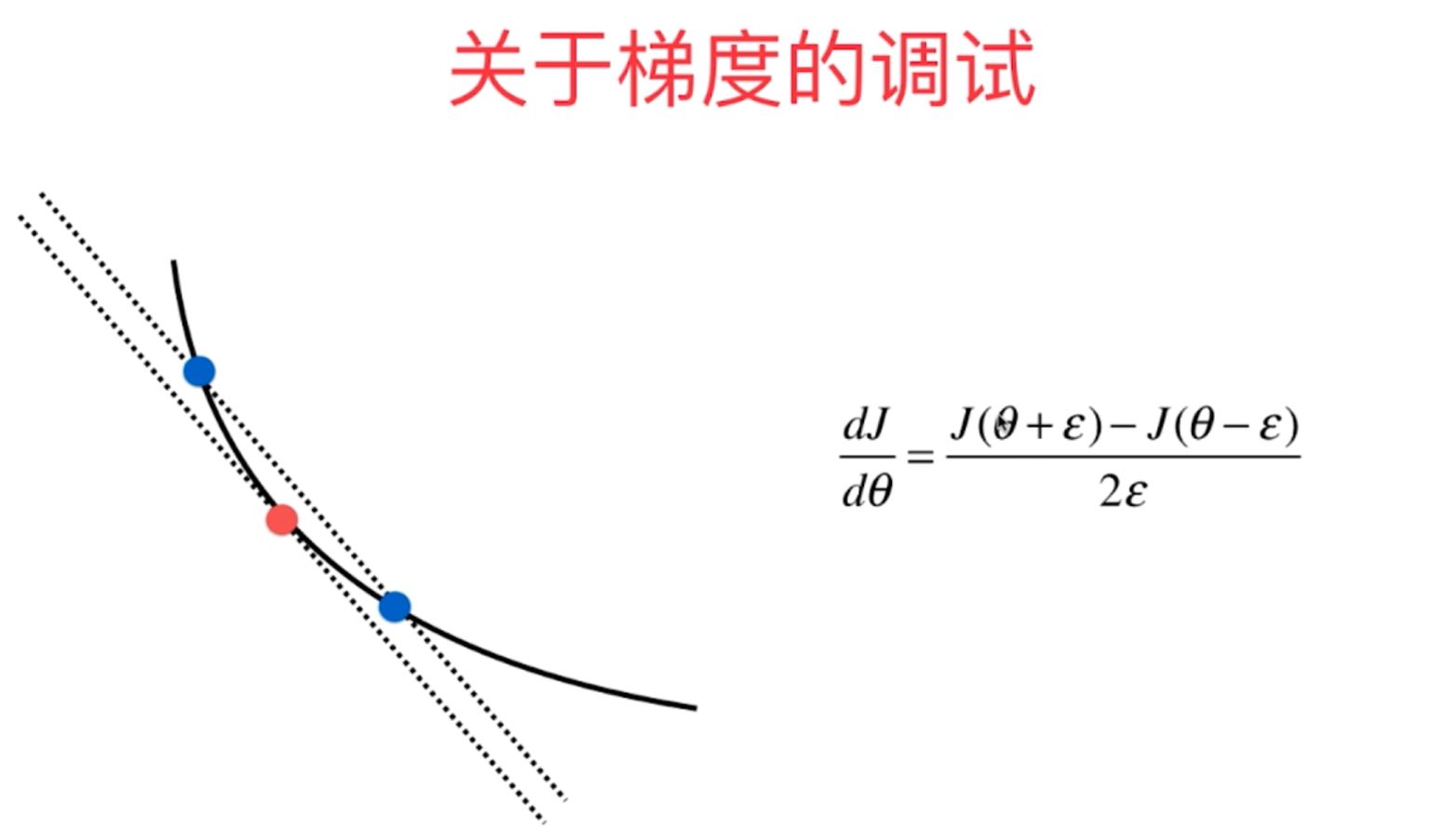
对于随机梯度法的调试，主要是对于损失函数的梯度的计算准确度的判断，即函数中关于各个参数偏导数DJ的计算，主要有两种方式：数学公式计算：利用多元函数的偏导计算，确定出其DJ的向量；（2）导数定义逼近法：利用逼近的方式进行各个参数偏导数的计算

其不同两种方式代码实现如下所示：
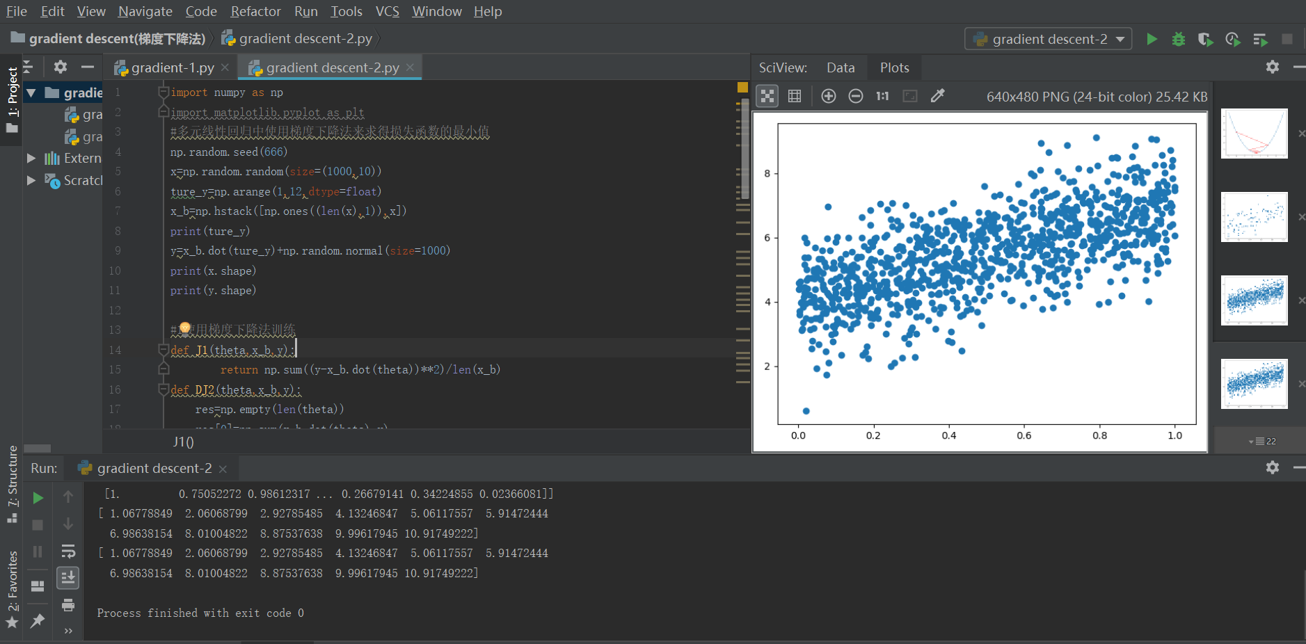
import numpy as np
import matplotlib.pyplot as plt
#多元线性回归中使用梯度下降法来求得损失函数的最小值
np.random.seed(666)
x=np.random.random(size=(1000,10))
ture_y=np.arange(1,12,dtype=float)
x_b=np.hstack([np.ones((len(x),1)),x])
print(ture_y)
y=x_b.dot(ture_y)+np.random.normal(size=1000)
print(x.shape)
print(y.shape)

#1使用梯度下降法训练
def J1(theta,x_b,y):
        return np.sum((y-x_b.dot(theta))**2)/len(x_b)
def DJ2(theta,x_b,y):
    res=np.empty(len(theta))
    res[0]=np.sum(x_b.dot(theta)-y)
    for i in range(1,len(theta)):
        res[i]=np.sum((x_b.dot(theta)-y).dot(x_b[:,i]))
    return res*2/len(x_b)
多元函数偏导数的计算方式

#1-1数学公式法

def DJmath(theta, x_b, y):
    return x_b.T.dot(x_b.dot(theta)-y)*2/len(y)

#1-2导数定义逼近法（各种函数都适用）

def DJdebug(theta, x_b, y,ep=0.0001):
    res = np.empty(len(theta))
    for f in range(len(theta)):
        theta1=theta.copy()
        theta1[f]=theta1[f]+ep
        theta2 = theta.copy()
        theta2[f] = theta2[f]-ep
        res[f]=(J1(theta1,x_b,y)-J1(theta2,x_b,y))/(2*ep)
    return res
def gradient_descent1(dj,x_b,y,eta,theta_initial,erro=1e-8, n=1e4):
    theta=theta_initial
    i=0
    while i<n:
        gradient =dj(theta,x_b,y)
        last_theta = theta
        theta = theta - gradient * eta
        if (abs(J1(theta,x_b,y) - J1(last_theta,x_b,y))) < erro:
            break
        i+=1
    return theta
print(x_b)
theta0=np.zeros(x_b.shape[1])
eta=0.1
theta1=gradient_descent1(DJdebug,x_b,y,eta,theta0)
print(theta1)
theta2=gradient_descent1(DJmath,x_b,y,eta,theta0)
print(theta2)