SSD: Single Shot MultiBox Detector论文阅读摘要

　　论文链接: https://arxiv.org/pdf/1512.02325.pdf

　　代码下载: https://github.com/weiliu89/caffe/tree/ssd

Abstract

We present a method for detecting objects in images using a single　deep neural network. Our approach, named SSD, discretizes the output space of　bounding boxes into a set of default boxes over different aspect ratios and scales　per feature map location
＃我们展示了一种使用单一深度神经网络的目标检测算法.我们的算法,又称SSD,将bounding boxes输出空间离散成一系列特征图上不同宽高比和尺度的default boxes.
At prediction time, the network generates scores for the presence of each object category in each default box and produces adjustments to the box to better match the object shape. Additionally, the network combines predictions from multiple feature maps with different resolutions to naturally handle objects of various sizes
#在预测阶段，网络根据每个default box中是否存在某种类别的物体进行评分，并调整box到更合适物体的形状.此外，网络融合多种不同分辨率特征图上的预测以适应不同尺寸的物体.
SSD is simple relative to methods that require object proposals because it completely eliminates proposal generation and subsequent pixel or feature resampling stages and encapsulates all computation in a single network. This makes SSD easy to train and straightforward to integrate into systems that require a detection component
#与那些需要obeject proposals的方法相比，SSD是简单的，因为它完全避免了proposal generation及随后的像素或特征重采样阶段，并将所有的计算都封装在单个网络．这使得SSD易于训练并以模块形式嵌入到检测系统中.
Experimental results on the PASCAL VOC, COCO, and ILSVRC datasets confirm that SSD has competitive accuracy to methods that utilize an additional object proposal step and is much faster, while providing a unified framework for both training and inference. For 300 × 300 input, SSD achieves 74.3% mAP1 on VOC2007 test at 59 FPS on a Nvidia TitanX and for 512 × 512 input, SSD achieves 76.9% mAP, outperforming a comparable state-of-the-art Faster R-CNN model. Compared to other single stage methods, SSD has much better accuracy even with a smaller input image size. Code is available at: https://github.com/weiliu89/caffe/tree/ssd
#PASCAL VOC,COCO以及ILSVRC数据集上的实验结果确认SSD相比那些需要额外object proposal阶段的方法更具有竞争力，在提供统一的训练和推理框架同时具有更快的运行速度．对于300*300输入分辨率，SSD在Nvida TitanX GPU上实现了59FPS以及74.3％的平均准确率，对于512*512的输入分辨率，SSD实现了76.9％的平均准确率，超过了同等情况下state-of-art Faster R-CNN模型.与其他单一阶段方法相比，SSD在使用更小输入分辨率的情况下实现了更高的准确率.代码可以在https://github.com/weiliu89/caffe/tree/ssd下载到

Introduction

Current state-of-the-art object detection systems are variants of the following approach:hypothesize bounding boxes, resample pixels or features for each box, and apply a high-quality classifier. This pipeline has prevailed on detection benchmarks since the Selective Search work [1] through the current leading results on PASCAL VOC, COCO, and ILSVRC detection all based on Faster R-CNN[2] albeit with deeper features such as[3]. While accurate, these approaches have been too computationally intensive for embedded systems and, even with high-end hardware, too slow for real-time applications
#当前的state-of-art目标检测系统是以下方法的变种：假定bounding box，为每个box进行像素或特征重采样，以及应用一个高质量的分类器．自从Selective Search[1]提出依赖，尽管文献[3]也用了更深的特征，PASCAL VOC，COCO和ILSVRC检测集上的领先实现都是基于Faster R-CNN[2].这个pipeline在图像benchmarks上盛行．尽管比较准确，这些方法对于嵌入式设备太占用运算资源，即使应用高端硬件，对于实时应用仍然太慢.
Often detection speed for these approaches is measured in seconds per frame (SPF),and even the fastest high-accuracy detector, Faster R-CNN, operates at only 7 frames per second (FPS). There have been many attempts to build faster detectors by attacking each stage of the detection pipeline (see related work in Sec. 4), but so far, significantly increased speed comes only at the cost of significantly decreased detection accuracy
#这些方法的检测速度通常是帧/秒(SPF)衡量的，即使是最快的高精度检测器，Faster R-CNN，只能运行在7帧/秒．研究人员通过优化检测pipeline的各个阶段作了很多努力，为了实现更快的检测器(见Section4相关作品)，但是至今检测速度的提高都建立在牺牲检测精度的基础上．
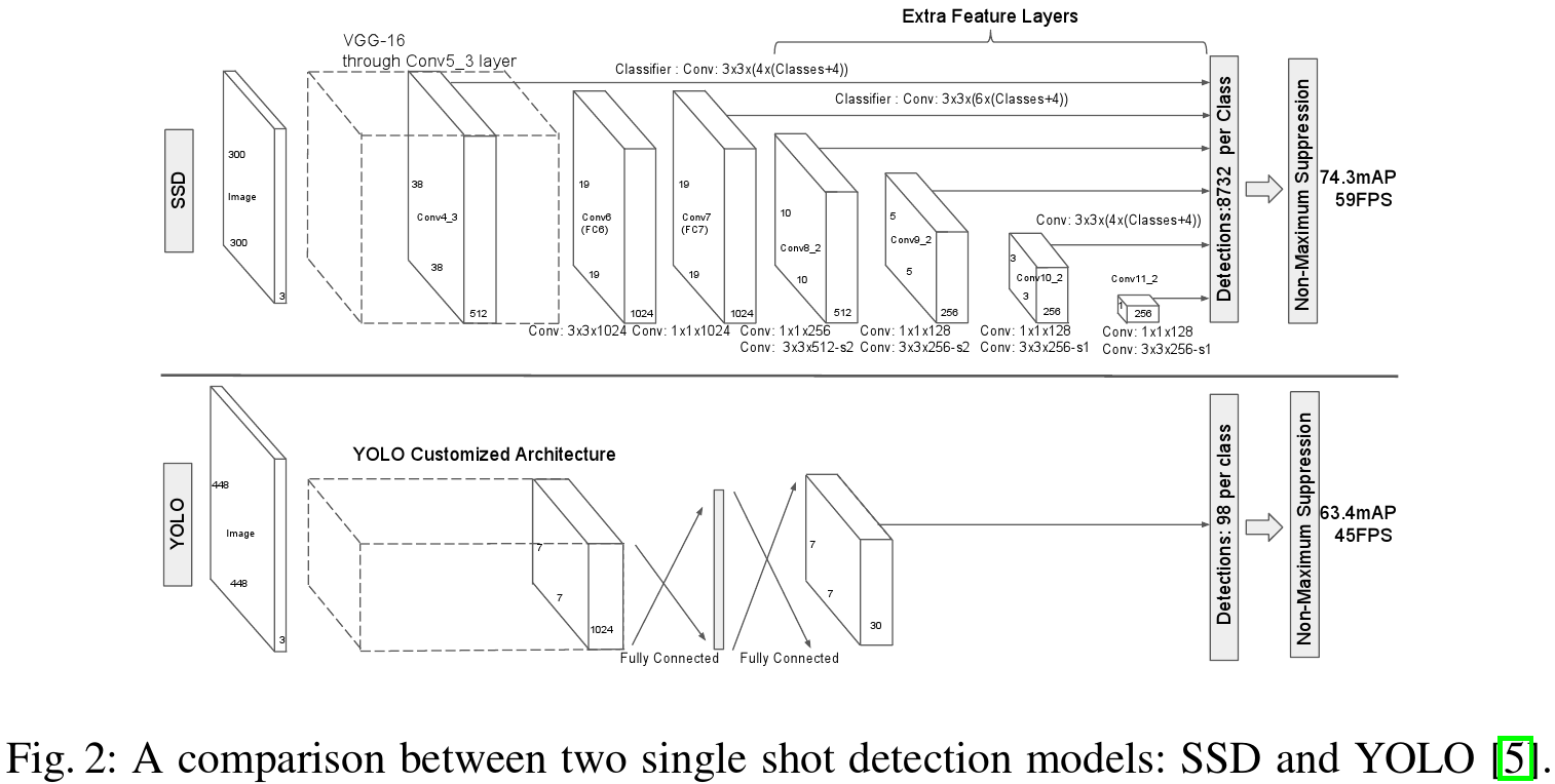
This paper presents the first deep network based object detector that does not resample pixels or features for bounding box hypotheses and and is as accurate as approaches that do. This results in a significant improvement in speed for high-accuracy detection (59 FPS with mAP 74.3% on VOC2007 test, vs. Faster R-CNN 7 FPS with mAP 73.2% or YOLO 45 FPS with mAP 63.4%). The fundamental improvement in speed comes from eliminating bounding box proposals and the subsequent pixel or feature resampling stage
＃本篇论文第一次展示了不需要对假定的bounding box进行像素或特征重采样的基于深度神经网络的目标检测器，并且仍然可以取得比较好的准确率．这促成了高精度检测算法在运行速度上的极大提升(VOC 2007 测试数据集74.3％的平均准确率，59FPS，对应的Faster R-CNN实现了73.2%的平均准确率，7FPS，YOLO实现63.4%的平均准确率,45FPS).速度提升改善的基础来源于消除了bounding box proposals及后续的像素和特征重采样阶段.
We are not the first to do this (cf [4,5]), but by adding a series of improvements, we manage to increase the accuracy significantly over previous attempts. Our improvements include using a small convolutional filter to predict object categories and offsets in bounding box locations, using separate predictors (filters) for different aspect ratio detections, and applying these filters to multiple feature maps from the later stages of a network in order to perform detection at multiple scales
#我们并非第一个这么做的(cf[4,5])，但是通过增加一系列的改进，相比先前的尝试显著提高了准确率．我们的改进包括使用一个小型卷积滤波器来预测物体类别以及bounding box坐标偏移，为不同的宽高比检测应用不同的滤波器，并将这些滤波器应用于后续的多尺度特征图，以实现不同尺度的检测．
With these modifications—especially using multiple layers for prediction at different scales—we can achieve high-accuracy using relatively low resolution input, further increasing detection speed. While these contributions may seem small independently, we note that the resulting system improves accuracy on real-time detection for PASCAL VOC from 63.4% mAP for YOLO to 74.3% mAP for our SSD. This is a larger relative improvement in detection accuracy than that from the recent, very high-profile work on residual networks [3]. Furthermore, significantly improving the speed of high-quality detection can broaden the range of settings where computer vision is useful
＃使用这些修改－－尤其针对不同尺度使用不同的层预测－－我们可以在相对低的分辨率下实现较高的准确率，进而提高检测速度．虽然这些修改看起来似乎有点毫无关联，我们注意到改进后的系统将PASCAL VOC实时检测的准确率从YOLO的63.4%提高到SSD的74.3%.这相比近期的高容量Res-Net[3]是一个极大的改善.进一步说，显著地提高了高质量检测器的速度可以扩展计算机视觉的应用范围.
We summarize our contributions as follows:
#将我们的贡献总结如下：
– We introduce SSD, a single-shot detector for multiple categories that is faster than the previous state-of-the-art for single shot detectors (YOLO), and significantly more accurate, in fact as accurate as slower techniques that perform explicit region proposals and pooling (including Faster R-CNN)
＃－我们引入了SSD，一个多目标检测的single-shot，比之前的state-of-the-art的single shot检测器(YOLO)更快，实际上达到了那些需要region proposals和pooling(包括Faster R-CNN)等更慢的算法一样的准确率．
– The core of SSD is predicting category scores and box offsets for a fixed set of default bounding boxes using small convolutional filters applied to feature maps
＃－SSD的核心是在卷积图上应用小卷积滤波器来预测分类得分以及一系列固定default bounding boxes的box偏置
– To achieve high detection accuracy we produce predictions of different scales from feature maps of different scales, and explicitly separate predictions by aspect ratio
＃－为了实现更高的准确率，我们针对不同尺度的特征图提出不同尺度的预测，并且根据宽高比进行预测的分离
– These design features lead to simple end-to-end training and high accuracy, even on low resolution input images, further improving the speed vs accuracy trade-off
＃－这些设计特征促使了简单的端到端训练以及低分辨率下的高准确率，进而改善了速度与准确率之间的权衡
– Experiments include timing and accuracy analysis on models with varying input size evaluated on PASCAL VOC, COCO, and ILSVRC and are compared to a range of recent state-of-the-art approaches
＃－使用PASCAL VOC, COCO以及ILSVRC数据集上不停输入尺寸对模型的实时性和准确率进行分析，并且与一系列state-of-the-art方法进行了比较

The Single Shot Detector (SSD)

This section describes our proposed SSD framework for detection (Sec. 2.1) and the associated training methodology (Sec. 2.2). Afterwards, Sec. 3 presents dataset-specific model details and experimental results
＃这一节描述了我们提出的SSD框架(节2.1)，随后，节３阐述了数据集的模型细节及实验结果


Fig. 1: SSD framework. (a) SSD only needs an input image and ground truth boxes for each object during training. In a convolutional fashion, we evaluate a small set (e.g. 4) of default boxes of different aspect ratios at each location in several feature maps with different scales (e.g. 8 × 8 and 4 × 4 in (b) and (c)). For each default box, we predict both the shape offsets and the confidences for all object categories ((c1 , c2 , · · · , cp )).At training time, we first match these default boxes to the ground truth boxes. For example, we have matched two default boxes with the cat and one with the dog, which are treated as positives and the rest as negatives. The model loss is a weighted sum between localization loss (e.g. Smooth L1 [6]) and confidence loss (e.g. Softmax)
＃图1:SSD框架.(a)SSD在测试阶段只需要输入图像和每个目标的ground truth boxes．在一个卷积fashion，我们对一小部分(例如４)不同尺度特征图(例如图b中的8*8以及图c中的4*4)对应的不同宽高比default boxes进行评估．对于每个default box,我们对那些default boxes的偏移量以及所有物体类别的置信度(c₁;c₂;......;c_p)进行预测．在训练阶段，我们首先将这些default boxes与ground truth boxes进行匹配．例如，我们将两个default boxes分别与猫和够进行匹配，这两个被当作正样本，其余的被当作负样本．模型的损失函数通过定位损失和分类损失进行衡量

2.1 Model

The SSD approach is based on a feed-forward convolutional network that produces a fixed-size collection of bounding boxes and scores for the presence of object class instances in those boxes, followed by a non-maximum suppression step to produce the final detections. The early network layers are based on a standard architecture used for high quality image classification (truncated before any classification layers), which we will call the base network2 . We then add auxiliary structure to the network to produce detections with the following key features:
#SSD算法基于一个可以产生固定尺寸bounding boxes集合和这些boxes上各类别得分的前向卷积网络,并通过非极大值抑制方法产生最后的检测结果.早期的网络层都是基于高质量图像分类的标准框架(分类层前截短),我们称之为基础网络2.然后我们在网络上增加辅助结构用于产生具有以下特征的检测结果:

Multi-scale feature maps for detection
#用于检测的多尺度特征图
We add convolutional feature layers to the end of the truncated base network. These layers decrease in size progressively and allow predictions of detections at multiple scales. The convolutional model for predicting detections is different for each feature layer (cf Overfeat[4] and YOLO[5] that operate on a single scale feature map).
#我们在截取后的基础网络末尾增加卷积特征层.这些层在尺寸上逐渐减少,因此允许多重尺度上的检测预测.每层特征层上的预测卷积模型都不一样(cf Overfeat[4] and YOLO[5]在单一尺度特征图上运行).

Convolutional predictors for detection
#用于检测的卷积预测器
Each added feature layer (or optionally an existing feature layer from the base network) can produce a fixed set of detection predictions using a set of convolutional filters. These are indicated on top of the SSD network architecture in Fig. 2
#每个增加的特征层(或可选的基础网络已存在的特征层)可以利用一系列卷积滤波器生成检测预测.图2中SSD网络结构顶层可以用于说明.
For a feature layer of size m × n with p channels, the basic element for predicting parameters of a potential detection is a 3 × 3 × p small kernel that produces either a score for a category, or a shape offset relative to the default box coordinates.At each of the m × n locations where the kernel is applied, it produces an output value. The bounding box offset output values are measured relative to a default box position relative to each feature map location (cf the architecture of YOLO[5] that uses an intermediate fully connected layer instead of a convolutional filter for this step).
#对于一个具有p通道尺寸为m*n的特征层,预测潜在检测(目标)的参数为3*3*p个小(卷积)核,用于预测类别的得分或者相对default box坐标系的形状偏移.在应用卷积核的m*n个位置中,都产生一个输出值.bounding box 偏移量输出值是基于每个特征图位置对应的fefault box位置(cf YOLO[5]结构在这一步中使用一个中间的全连接层替代卷积核).


Our SSD model adds several feature layers to the end of a base network, which predict the offsets to default boxes of different scales and aspect ratios and their associated confidences. SSD with a 300 × 300 input size significantly outperforms its 448 × 448 YOLO counterpart in accuracy on VOC2007 test while also improving the speed.
#我们的SSD模型在基础网络末尾增加了一些特征层,用于预测相对不同尺度及宽高比default boxes的偏移量以及对应的置信度.使用VOC2007测试集验证,SSD使用300*300输入尺寸在准确率上完胜YOLO使用448*448输入尺寸,同时也具有更快的速度.


Default boxes and aspect ratios
#Default boxes和宽高比
We associate a set of default bounding boxes with each feature map cell, for multiple feature maps at the top of the network. The default boxes tile the feature map in a convolutional manner, so that the position of each box relative to its corresponding cell is fixed. At each feature map cell, we predict the offsets relative to the default box shapes in the cell, as well as the per-class scores that indicate the presence of a class instance in each of those boxes. Specifically, for each box out of k at a given location, we compute c class scores and the 4 offsets relative to the original default box shape.
#我们为网络顶端的多重特征图上的每个特征图单元假定了一系列default bounding boxes,default boxes以卷积形式覆盖整个特征图,因此每个box相对其对应单元的位置是固定的.在每个特征图单元上,我们预测相对于单元中default box的偏置量,以及用于指示每个boxes中是否存在各类别的per-class得分.特别的,对于给定位置k个box中的其中之一,我们计算c个分类得分以及4个相对原始default box 的偏置量.
This results in a total of (c + 4)k filters that are applied around each location in the feature map, yielding (c + 4)kmn outputs for a m × n feature map. For an illustration of default boxes, please refer to Fig. 1. Our default boxes are similar to the anchor boxes used in Faster R-CNN [2], however we apply them to several feature maps of different resolutions. Allowing different default box shapes in several feature maps let us efficiently discretize the space of possible output box shapes.
#在特征图每个位置周围实际应用了(c+4)*k个滤波器,进而在一个m*n特征图上对应(c+4)*kmn输出.关于default boxes的说明请参考图1.我们的default boxes类似于Faster R-CNN[2]中用到的anchor boxes,但是我们将他们应用到一些不同分辨率的特征图中.在这些特征图中使用不同的default box 允许我们有效率的离散潜在输出box形状的空间.

2.2 Training

The key difference between training SSD and training a typical detector that uses region proposals, is that ground truth information needs to be assigned to specific outputs in the fixed set of detector outputs. Some version of this is also required for training in YOLO[5] and for the region proposal stage of Faster R-CNN[2] and MultiBox[7]. Once this assignment is determined, the loss function and back propagation are applied end-to-end. Training also involves choosing the set of default boxes and scales for detection as well as the hard negative mining and data augmentation strategies.
#训练SSD和基于region proposals的经典检测器的重要差别在于,ground-truth 信息需要被分配到一系列固定检测器输出结果中.有一些版本的YOLO[5]的训练以及Faster R-CNN[2]的region proposal阶段以及MultiBox[7]也需要执行上述动作.一旦完成了分配,损失函数及反向传播实现了端到端应用.训练也包含default boxes集合的选择,用于检测的尺度以及hard negative mining以及数据增广策略.

Matching strategy
#匹配策略
During training we need to determine which default boxes correspond to a ground truth detection and train the network accordingly. For each ground truth box we are selecting from default boxes that vary over location, aspect ratio, and scale. We begin by matching each ground truth box to the default box with the best jaccard overlap (as in MultiBox [7]). Unlike MultiBox, we then match default boxes to any ground truth with jaccard overlap higher than a threshold (0.5). This simplifies the learning problem, allowing the network to predict high scores for multiple overlapping default boxes rather than requiring it to pick only the one with maximum overlap.
#在训练阶段我们需要决定哪个default boxes与ground truth检测相关,并对应的训练网络.对于每个ground truth box我们需要从不同位置,宽高比,尺度中挑选default boxes.我们开始将每个ground truth box与具有最佳jaccard overlap(如文献7中所述MultiBox)的default box进行匹配.与MultiBox不同的是,我们之后将default boxes与任意jaccard overlap超过阈值(0.5)的ground truth进行匹配.这简化了学习问题,允许网络为多重overlapping default boxes 预测高的得分,而不是需要只选择具有最高overlap的default box.

Training objective
#训练目标
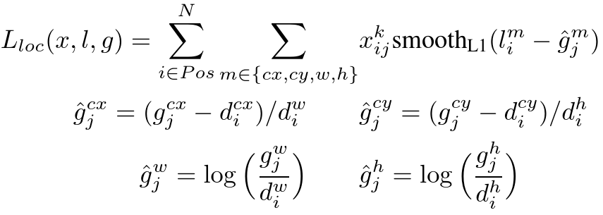
The SSD training objective is derived from the MultiBox objective [7,8] but is extended to handle multiple object categories.Let x^p_ij = {1, 0} be an indicator for matching the i-th default box to the j-th ground truth box of category p.In the matching strategy above, we can have ∑_i x^p_ij≥ 1.The overall objective loss function is a weighted sum of the localization loss (loc) and the confidence loss (conf):
##SSD训练目标由MultiBox objective[7,8]沿用,但作了一些扩展用于处理多种目标类别.假定x^p_ij= {1, 0}为第i个default box与类别p的第j个ground truth box时候匹配.在上述的匹配策略中,我们可以得到 ∑_i x^p_ij≥ 1.总体的目标损失函数由定位损失和分类损失的加权得到:

where N is the number of matched default boxes. If N = 0, wet set the loss to 0. The localization loss is a Smooth L1 loss [6] between the predicted box (l) and the ground truth box (g) parameters. Similar to Faster R-CNN [2], we regress to offsets for the center (cx, cy) of the default bounding box (d) and for its width (w) and height (h).
#其中N是匹配的default boxes的数量．如果N=0,我们设置损失为0．定位损失是一个预测框(l)和ground truth box(g)之间的平滑L1损失[6]．与Faster R-CNN [2]类似，我们将default bounding box的中心点坐标(cx,cy)以及它的宽和高作为回归．


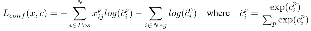
The confidence loss is the softmax loss over multiple classes confidences (c).

and the weight term α is set to 1 by cross validation.

Choosing scales and aspect ratios for default boxes
＃为default boxes选择尺度和宽高比
To handle different object scales,some methods [4,9] suggest processing the image at different sizes and combining the　results afterwards. However, by utilizing feature maps from several different layers in a　single network for prediction we can mimic the same effect, while also sharing parameters across all object scales. Previous works [10,11] have shown that using feature maps　from the lower layers can improve semantic segmentation quality because the lower　layers capture more fine details of the input objects.
＃为了处理不同尺寸的目标，有一些方法[4,9]建议以不同的尺寸处理图像，随后将结果混合在一起．但是，通过利用单一网络中不同网络层中用于预测的特征图的方式我们也可以达到相同的效果，同时也实现所有目标尺度上的权值共享．早期的作品[10,11]也展示了使用更低层次的网络层特征图可以改善语义分割质量，因为更低层网络包含输入物体的更多细节
Similarly, [12] showed that adding　global context pooled from a feature map can help smooth the segmentation results.Motivated by these methods, we use both the lower and upper feature maps for detection.Figure 1 shows two exemplar feature maps (8*8 and 4*4) which are used in the framework. In practice, we can use many more with small computational overhead.
#类似的，文献[12]展示了通过增加特征图池化得到的全局语境有助于平滑分割结果．受这些方法启发，我们使用了低层次和高层次的特征图用于检测．图1展示了框架中使用的两个特征图原型(8*8及4*4).实践中，由于计算开销比较小，我们可以使用更多．
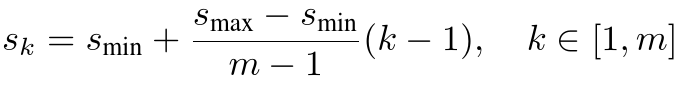
Feature maps from different levels within a network are known to have different　(empirical) receptive field sizes [13]. Fortunately, within the SSD framework, the default boxes do not necessary need to correspond to the actual receptive fields of each　layer. We design the tiling of default boxes so that specific feature maps learn to be　responsive to particular scales of the objects. Suppose we want to use m feature maps　for prediction. The scale of the default boxes for each feature map is computed as:
#同一个网络里面不同层次的特征图被认为[13]拥有不同的感受野.幸运的是,在SSD框架内,default boxes不需要与每层的实际感受野相对应．我们设计了default boxes的tiling，因此特定的特征图被训练与特征尺寸的目标相关．假设我们在检测任务中使用m个特征图.每个特征图的default boxes的尺寸计算如下:

where s_min is 0.2 and s_max is 0.9, meaning the lowest layer has a scale of 0.2 and the highest layer has a scale of 0.9, and all layers in between are regularly spaced.We impose different aspect ratios for the default boxes,and denote them as α_r∈{1,2,3,1/2,1/3}.We can compute the width (w^a_k = s_k√a_r) and height (h^a_k = s_k/√a_r) for each default box.For the aspect ratio of 1, we also add a default box whose scale is s'_k = √s_ks_k+1,resulting in 6 default boxes per feature map location.We set the center of each default box to ((i+0.5)/|f_k|,(j+0.5)/|f_k|),where |f_k| is the size of the k-th square feature map, i, j ∈ [0,|f_k|).In practice, one can also design a distribution of default boxes to best fit a specific dataset. How to design the optimal tiling is an open question as well.
#其中smin等于0.2,smax等于0.9,意味着最低层尺度为0.2,最高层尺度为0.9,所有网络层都空间有序排列.我们为default boxes施加不同宽高比,并指代它们为α_r∈{1,2,3,1/2,1/3}.我们为每个default box计算宽度(w^a_k = s_k√a_r)和高度(h^a_k = s_k/√a_r)．对于宽高比为１，我们增加了一个尺度为s'_k = √s_ks_k+1的default box,因此每个特征图位置包含6个default boxes.我们设置default box的中心为((i+0.5)/|f_k|,(j+0.5)/|f_k|),其中|f_k|是第ｋ个方形特征图的尺寸，i, j ∈ [0,|f_k|).实践上,也可以设计default boxes的分布为最适合数据集的．如果设计优化最优覆盖仍然是个开放的问题．

Hard negative mining
By combining predictions for all default boxes with different scales and aspect ratios from all locations of many feature maps, we have a diverse set of predictions, covering various input object sizes and shapes. For example, in Fig. 1, the dog is matched to a default box in the 4 × 4 feature map, but not to any default boxes in the 8 × 8 feature map.This is because those boxes have different scales and do not match the dog box,and therefore are considered as negatives during training
#通过将许多特征图各位置上不同尺度和宽高比default boxes的预测混合在一起,我们得到一个多样化的预测集,涵盖各种不同的输入目标尺寸和形状.例如在图1中,狗与4*4特征图中的default box相匹配,但是并不是任何8*8中的default boxes.这是因为那些boxes拥有不同的尺度,并不匹配狗的形状,因此在训练时被当做负样本
After the matching step, most of the default boxes are negatives, especially when the number of possible default boxes is large. This introduces a significant imbalance between the positive and negative training examples. Instead of using all the negative examples, we sort them using the highest confidence loss for each default box and pick the top ones so that the ratio between the negatives and positives is at most 3:1. We found that this leads to faster optimization and a more stable training
#在匹配阶段之后,大多数default boxes都是负样本,尤其是当潜在的default boxes数量很大时.这引入了正样本和负样本之间的严重不平衡.我们使用最高的confidence loss 为每个default box进行排序并选择前几个负样本,因此负样本与正样本的比值在大多数情况下为3:1,而不是直接使用负样本.我们发现这促使更快的优化以及更稳定的训练

Data augmentation
To make the model more robust to various input object sizes and shapes, each training image is randomly sampled by one of the following options
- Use the entire original input image.
- Sample a patch so that the minimum jaccard overlap with the objects is 0.1, 0.3, 0.5, 0.7, or 0.9.
- Randomly sample a patch.
The size of each sampled patch is [0.1, 1] of the original image size, and the aspect ratio is between 12 and 2. We keep the overlapped part of the ground truth box if the center of it is in the sampled patch. After the aforementioned sampling step, each sampled patch is resized to fixed size and is horizontally flipped with probability of 0.5, in addition to applying some photo-metric distortions similar to those described in [14]
#为了使模型对各种不同尺寸及形状输入目标具有更高的鲁棒性,每个训练样本都经过以下其中之一方式随机采样:
- 使用整张原始输入图像
- 采样patch因此最小的jaccard overlap为 0.1, 0.3, 0.5, 0.7, or 0.9
- patch随机采样
每个采样的patch的尺寸为原始图像的[0.1,1],宽高比在1/2到2之间.我们会保留ground truth box的overlapped部分,如果它的中心在被采样的patch中.在上述采样阶段之后，每个采样的patch被缩放到固定尺寸,并以0.5的概率作水平翻转,为了处理类似文献[14]描述的photo-metric分布

　　Experimental Results

Base network

Our experiments are all based on VGG16 [15], which is pre-trained on the ILSVRC CLS-LOC dataset [16]. Similar to DeepLab-LargeFOV [17], we convert fc6 and fc7 to convolutional layers, subsample parameters from fc6 and fc7, change pool5 from 2 × 2 − s2 to 3 × 3 − s1,and use the à trous algorithm [18] to fill the ”holes”. We remove all the dropout layers and the fc8 layer. We fine-tune the resulting model using SGD with initial learning rate 10−3 , 0.9 momentum, 0.0005 weight decay, and batch size 32.The learning rate decay policy is slightly different for each dataset, and we will describe details later. The full training and testing code is built on Caffe [19] and is open source at: https://github.com/weiliu89/caffe/tree/ssd.
#我们的实验都是基于VGG16[15],并在ILSVRC CLS-LOC数据集[16]上预训练.类似于DeepLab-LargeFOV[17],我们把fc6和fc7转换为卷积层,对fc6和fc7中的参数进行二次采样,将pool5从2*2-s2更改到3*3-s1,并使用à trous algorithm[18]补这个"窟窿".我们移除了所有的dropout层以及fc8层.我们使用10-3的初始学习率,0.9的momentum,0.0005的weight decay以及32的batch size,通过SGD对模型进行fine-tune.所有的训练和测试代码都是基于Caffe[19],并可以在https://github.com/weiliu89/caffe/tree/ssd开放下载

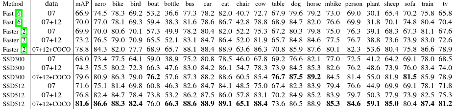
3.1 PASCAL VOC2007

On this dataset, we compare against Fast R-CNN [6] and Faster R-CNN [2] on VOC2007 test (4952 images). All methods fine-tune on the same pre-trained VGG16 network.
#在这个数据集上，我们对比了SSD与Fast R-CNN[6]和Faster R-CNN[2]在VOC2007测试集(4952张图片)上的表现．所有的方法都是就要VGG16预训练模型进行fine-tune.
Figure 2 shows the architecture details of the SSD300 model. We use conv4_3,conv7 (fc7), conv8_2, conv9_2, conv10_2, and conv11_2 to predict both location and confidences. We set default box with scale 0.1 on conv4_3.We initialize the parameters for all the newly added convolutional layers with the ”xavier” method[20].For conv4_3,conv10_2 and conv11_2, we only associate 4 default boxes at each feature map location – omitting aspect ratios of 1/3 and 3.
#图2展示了SSD300模型的结构细节.我们使用conv4_3,conv7 (fc7), conv8_2, conv9_2, conv10_2, and conv11_2来预测定位和置信度.我们设置conv4_3上的default box尺度为0.1.我们使用"xavier"方法对新增卷积层参数进行初始化.对于conv4_3,conv10_2及conv11_2,我们在每个特征图位置上配置4个default box -- 忽略宽高比为1/3和3．
For all other layers, we put 6 default boxes as described in Sec. 2.2. Since, as pointed out in [12], conv4_3 has a different feature scale compared to the other layers, we use the L2 normalization　technique introduced in [12] to scale the feature norm at each location in the feature map to 20 and learn the scale during back propagation. We use the 10⁻³ learning rate for 40k iterations, then　continue training for 10k iterations with 10⁻⁴ and 10⁻⁵. When training on VOC2007 trainval, Table 1 shows that our low resolution SSD300 model is already more accurate than Fast R-CNN
#对于其他所有网络层，我们放置了sec 2.2描述的6个default boxes.因此，如文献[12]指出的,conv4_3拥有与其他层不一样的尺度,我们使用文献[12]中描述的L2正则化将特征图上每个位置的特征量化到20,并在反向传播中学习尺度.我们使用10-3的学习率训练了40k个iterations,之后使用10−4及10−5继续训练了10k个iterations.在VOC2007 trainval训练时，表1表明我们的低分辨率SSD300模型已经比Fast R-CNN更准确
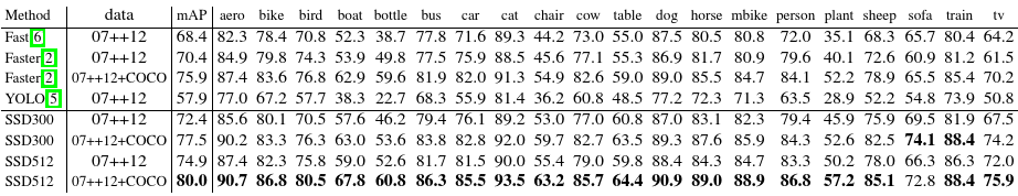
When we train SSD on a larger 512 × 512 input image, it is even more accurate, surpassing Faster R-CNN by 1.7% mAP. If we train SSD with more (i.e. 07+12) data, we see that SSD300 is already better than Faster R-CNN by 1.1% and that SSD512 is 3.6% better. If we take models trained on COCO trainval35k as described in Sec. 3.4 and fine-tuning them on the 07+12 dataset with SSD512, we achieve the best results: 81.6% mAP
#当我们使用SSD在一个更大的512*512的输入图像上训练时,它变得更精确,比Faster R-CNN 高了1.7%.如果使用更多训练数据(例如07+12),我们可以发现SSD300在平均准确率上已经高出Faster R-CNN　1.1％,同时SSD512高出3.6%.如果我们在Sec 3.4中描述的COCO trainval35k训练模型,并使用SSD512在07+12数据集上进行fine-tuning,我们实现了最佳的结果:81.6%
To understand the performance of our two SSD models in more details, we used the detection analysis tool from [21]. Figure 3 shows that SSD can detect various object categories with high quality (large white area). The majority of its confident detections are correct. The recall is around 85-90%, and is much higher with “weak” (0.1 jaccard overlap) criteria
#为了理解两个SSD模型的更多细节,我们使用文献[21]中的检测分析工具.表3说明SSD可以高质量的检测各种物体类别.大多数检测都是正确的.recall数值在85-90%,使用弱的检测标准时将具有更高的recall值
Compared to R-CNN [22], SSD has less localization error, indicating that SSD can localize objects better because it directly learns to regress the object shape and classify object categories instead of using two decoupled steps. However, SSD has more confusions with similar object categories (especially for animals), partly because we share locations for multiple categories. Figure 4 shows that SSD is very sensitive to the bounding box size. In other words, it has much worse performance on smaller objects than bigger objects
#相比与文献[22]中的R-CNN，SSD具有更少的定位错误，说明SSD可以更好的定位物体，因为它直接学习如何对物体形状进行回归并对物体类别进行分类而不是使用两个独立的步骤.但是，SSD对近似的物体类别更为困惑，部分原因可能是多个类别共享定位.图4说明SSD对bounding box尺寸非常敏感.换句话说,它在小物体检测上表现的没有大物体好
This is not surprising because those small objects may not even have any information at the very top layers. Increasing the input size (e.g. from 300 × 300 to 512 × 512) can help improve detecting small objects, but there is still a lot of room to improve. On the positive side, we can clearly see that SSD performs really well on large objects. And it is very robust to different object aspect ratios because we use default boxes of various aspect ratios per feature map location
#这并不令人惊讶,因为那些小的物体在最顶层可能没有任何信息．提高输入尺寸(例如从300*300到512*512)有助于提高检测细小物体，但是仍然有提高空间.在positive side上，我们可以清晰的看到SSD在大物体上表现的非常好.而且它对不同目标宽高比具有很好的鲁棒性，因为我们在每个特征图位置上使用各种宽高比的default boxes

Table 1: PASCAL VOC2007 test detection results.
Both Fast and Faster R-CNN use input images whose minimum dimension is 600. The two SSD models have exactly the same settings except that they have different input sizes (300×300 vs. 512×512). It is obvious that larger input size leads to better results, and more data always helps. Data: ”07”: VOC2007 trainval, ”07+12”: union of VOC2007 and VOC2012 trainval.”07+12+COCO”: first train on COCO trainval35k then fine-tune on 07+12
＃Fast和Faster R-CNN使用最小维数为600的输入数据.这两个SSD模型除了输入尺寸(300*300 Vs 512*512)以外具有完全相同的设置．很明显更大的输入尺寸促使更好的结果，更多的数据同样有助于.数据＂07＂代表VOC2007 trainval,数据＂07+12＂代表VOC2007和VOC2012 trainval的联合数据集,数据"07+12+COCO"代表 首先在COCO trainval35k 上测试，然后在VOC2007和VOC2012 trainval的联合数据集上fine-tune

3.2 Model analysis

To understand SSD better, we carried out controlled experiments to examine how each component affects performance. For all the experiments, we use the same settings and input size (300 × 300), except for specified changes to the settings or component(s)
#为了更好的理解SSD,我们使用对照实验来验证每个模块是如何影响表现的.对于所有的实验，我们都使用相同的设置以及输入尺寸(300*300),除了特定的设置变更或模块.

Table 2: Effects of various design choices and components on SSD performance
＃表２:不同设计选择及模块对SSD表现的影响

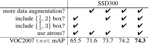
Data augmentation is crucial
＃数据增广是重要的
Fast and Faster R-CNN use the original image and the horizontal flip to train. We use a more extensive sampling strategy, similar to YOLO [5].Table 2 shows that we can improve 8.8% mAP with this sampling strategy. We do not know how much our sampling strategy will benefit Fast and Faster R-CNN, but they are likely to benefit less because they use a feature pooling step during classification that is relatively robust to object translation by design
＃Fast以及Faster R-CNN使用原始图像以及水平翻转图像进行测试.我们使用了一种更为昂贵的采样策略,类似于文献[5]中的YOLO.表２说明使用这个采样策略可以提高8.8％的平均准确率.我们不知道这个策略能多大程度上改善Fast以及Faster R-CNN，但是似乎帮助不大，因为它们在分类阶段使用了池化操作，因此设计上对物体平移具有更高的鲁棒性.


Fig. 3: Visualization of performance for SSD512 on animals, vehicles, and furniture from VOC2007 test
＃图３　SSD512在VOC2007测试集 动物,汽车,家具的表现可视化
The top row shows the cumulative fraction of detections that are correct (Cor) or false positive due to poor localization (Loc), confusion with similar categories (Sim), with others (Oth), or with background (BG). The solid red line reflects the change of recall with strong criteria (0.5 jaccard overlap) as the number of detections increases. The dashed red line is using the weak criteria (0.1 jaccard overlap). The bottom row shows the distribution of top-ranked false positive types
＃第一行展示了检测的cumulative fraction(累积分布函数),其中正确与否取决于poor localization (Loc),confusion with similar categories (Sim),以及others (Oth),或者background (BG).红色的实线反应了检测数量增加时,强标准(0.5 jaccard overlap)带来recall的变换.最后一行展示了top-ranked false positive types的分布

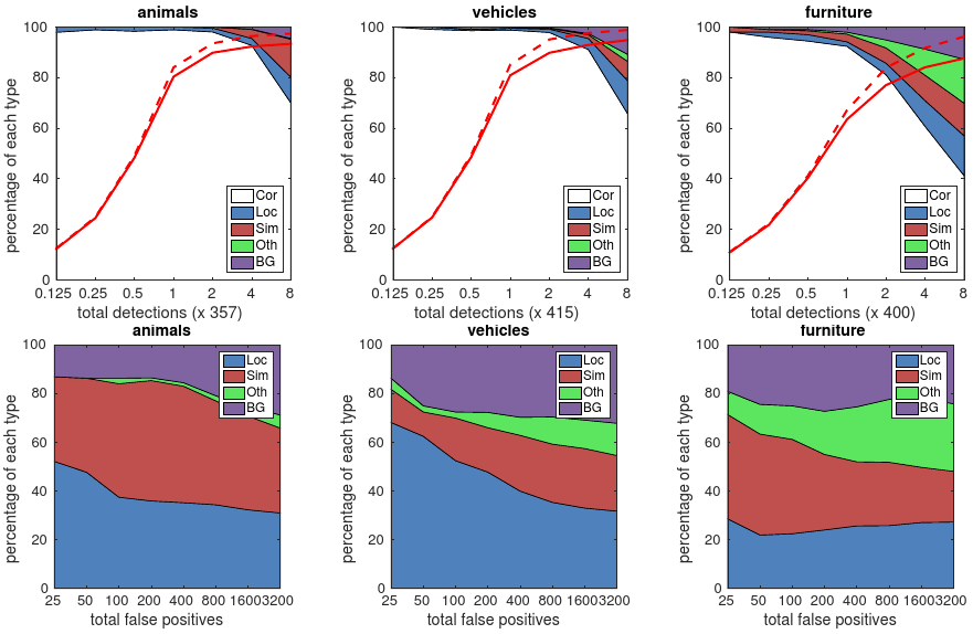
　Fig. 4: Sensitivity and impact of different object characteristics on VOC2007 test set using [21]

　＃VOC2007数据集上使用文献[21]所述方法对不同物体特性的影响.

　The plot on the left shows the effects of BBox Area per category, and the right plot shows the effect of Aspect Ratio. Key: BBox Area: XS=extra-small;S=small; M=medium; L=large; XL =extra-large. Aspect Ratio: XT=extra-tall/narrow;T=tall; M=medium; W=wide; XW =extra-wide

　#左边的曲线展示了每个类别上BBox Area的影响，右边的曲线展示了Aspect Ration的影响．关键词:BBox Area:XS=XS=extra-small;S=small; M=medium; L=large; XL =extra-large.Aspect Ratio: XT=extra-tall/narrow;T=tall; M=medium; W=wide; XW =extra-wide

　　　More default box shapes is better

More default box shapes is better. As described in Sec. 2.2, by default we use 6 default boxes per location. If we remove the boxes with 1/3 and 3 aspect ratios, the performance drops by 0.6%. By further removing the boxes with 1/2 and 2 aspect ratios,the performance drops another 2.1%. Using a variety of default box shapes seems to make the task of predicting boxes easier for the network
#如Sec.2.2描述的一样，默认情况下我们在每个位置使用6个default boxes．如果我们把宽高比为1/3和3的boxes移去，准确率会下降0.6%，进一步移去宽高比为1/2和2的boxes,准确率会进一步下降2.1%，使用多种default box shapes 看起来使预测boxes更适合工作

　　　Atrous is faster

As described in Sec. 3, we used the atrous version of a subsampled VGG16, following DeepLab-LargeFOV [17]. If we use the full VGG16, keeping pool5 with 2 × 2 − s2 and not subsampling parameters from fc6 and fc7, and add conv5 3 for prediction, the result is about the same while the speed is about 20% slower
＃如Sec.3.3描述的一样，我们在DeepLab-LargeFOV[17]后面使用VGG16下采样的一个atrous版本．如果我们使用完整的VGG16,保留pool5和2*2-s2，不从fc6和fc7中降采样，并增加conv5_3用于预测，结果几乎相同但是速度降低了20%.

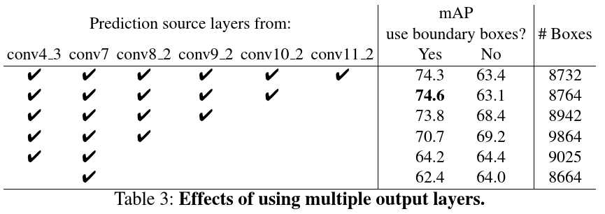
　　　Multiple output layers at different resolutions is better

A major contribution of SSD is using default boxes of different scales on different output layers. To measure the advantage gained, we progressively remove layers and compare results. For a fair comparison, every time we remove a layer, we adjust the default box tiling to keep the total number of boxes similar to the original (8732). This is done by stacking more scales of boxes on remaining layers and adjusting scales of boxes if needed. We do not exhaustively optimize the tiling for each setting
＃SSD的一个主要贡献是使用不同尺度的default boxes．为了衡量这个策略带来多大的改善，我们逐步移除网络层并对比其结果．为了实现公平对比，每次我们移除一个网络层，需要对default boxes tiling进行调整到剩余boxes数量接近原网络(8732).这是通过在剩余网络层附加更多的boxes，并在可能的时候调整boxes的尺度．我们不需要把每个设置都调整到最优．
Table 3 shows a decrease in accuracy with fewer layers, dropping monotonically from 74.3 to 62.4.When we stack boxes of multiple scales on a layer, many are on the image boundary and need to be handled carefully. We tried the strategy used in Faster R-CNN [2], ignoring boxes which are on the boundary. We observe some interesting trends. For example, it hurts the performance by a large margin if we use very coarse feature maps (e.g. conv11 2 (1 × 1) or conv10 2 (3 × 3)). The reason might be that we do not have enough large boxes to cover large objects after the pruning. 
＃表３展示了减少网络层带来的平均准确率的下降，从74.3%下降到62.4%.当我们将不同尺度的boxes附加到一个网络层上时，很多会在图像的边缘上，因此需要仔细处理．我们尝试了Faster R-CNN[2]使用的策略，忽略边界上的boxes.我们发现了一些有趣的趋势．举个例子，如果我们使用非常coarse的特征图(例如conv11_2(1*1)或(conv10_2(3*3)))，将会在很大程度上影响性能，原因可能是我们没有足够大的boxes来覆盖pruning(剪枝)的大目标．
When we use primarily finer resolution maps, the performance starts increasing again because even after pruning a sufficient number of large boxes remains. If we only use conv7 for prediction, the performance is the worst,reinforcing the message that it is critical to spread boxes of different scales over different layers. Besides, since our predictions do not rely on ROI pooling as in [6], we do not have the collapsing bins problem in low-resolution feature maps [23]. The SSD architecture combines predictions from feature maps of various resolutions to achieve comparable accuracy to Faster R-CNN, while using lower resolution input images.
＃当我们使用主要finer(好的，出色的)分辨率的特征图时，准确率重新开始增加，因为即使在pruning(剪枝)之后仍然有一大部分boxes被保留.如果我们使用conv7来预测，表现是最差的，这强调了必须在不同层使用不同尺寸的boxes的信念．此外，因为我们的预测不依赖于文献[6]提到的ROI pooling，所以我们不存在低分辨率特征图中的collapsing bin问题．SSD结构融合了特征图中不同分辨率的预测结果来实现与Faster R-CNN类似的准确率，尤其是使用低分辨率图像时.

3.3 PASCAL VOC2012

We use the same settings as those used for our basic VOC2007 experiments above,except that we use VOC2012 trainval and VOC2007 trainval and test (21503　images) for training, and test on VOC2012 test (10991 images). We train the models with 10⁻³ learning rate for 60k iterations, then 10⁻⁴ for 20k iterations. Table 4 shows the results of our SSD300 and SSD5124 model. We see the same performance trend as we observed on VOC2007 test. Our SSD300 improves accuracy over Fast/Faster R-CNN. By increasing the training and testing image size to 512 × 512, we are 4.5% more accurate than Faster R-CNN. Compared to YOLO, SSD is significantly more accurate,likely due to the use of convolutional default boxes from multiple feature maps and our matching strategy during training. When fine-tuned from models trained on COCO, our SSD512 achieves 80.0% mAP, which is 4.1% higher than Faster R-CNN
#我们使用与基础VOC2007实验相同的配置，除了我们使用VOC2012 trainval及VOC2007 trainval数据集和test数据集(21503张图像)以及VOC2012 test数据集(10991张图像)．我们使用10^-3的学习率训练了60k个iterations，随后使用10^-4的学习率训练了20k个iterations.表4展示了我们的SSD300和SSD512⁴上的结果．我们可以看到类似于VOC2007 test数据集上类似的性能趋势．我们的SSD300在性能上超越了Fast/Faster R-CNN.通过把训练和测试图像尺寸提高到512*512，我们的平均准确率比Faster R-CNN提高了4.5%．相比于YOLO,SSD明显更加准确，可能是因为使用了复合特征图上的卷积default boxes和我们训练阶段的匹配策略．对COCO数据集上训练的模型进行fine-tuned，我们的SSD512实现了80.0%的平均准确率，比Faster R-CNN高出了4.1%.
Table 4: PASCAL VOC2012 test detection results. Fast and Faster R-CNN use images with minimum dimension 600, while the image size for YOLO is 448 × 448. data: ”07++12”: union of VOC2007 trainval and test and VOC2012 trainval. ”07++12+COCO”: first train on COCO trainval35k then fine-tune on 07++12
＃表４：PASCAL VOC2012测试检测结果.Fast和Faster R-CNN使用最小纬度为600的图像，而YOLO使用的图像尺寸为448*448.数据:"07++12"：VOC2007 trainval和test数据集以及VOC2012 trainval数据集."07++12+COCO"：首先在COCO trainval35k数据集上训练然后在07++12数据集上fine-tune.

3.4 COCO

To further validate the SSD framework, we trained our SSD300 and SSD512 architectures on the COCO dataset. Since objects in COCO tend to be smaller than PASCAL VOC, we use smaller default boxes for all layers. We follow the strategy mentioned in Sec. 2.2, but now our smallest default box has a scale of 0.15 instead of 0.2, and the scale of the default box on conv4 3 is 0.07 (e.g. 21 pixels for a 300 × 300 image)⁵＃为了进一步验证SSD框架，我们在COCO数据集上训练了SSD300和SSD512结构．由于COCO数据集上的目标通常比PASCAL VOC数据集上更小，我们在所有层上使用了更小的default boxes．我们遵循Sec2.2中提到的策略，但是现在我们最小的default box尺寸为0.15而不是0.2，同时conv4_3上default box的尺寸是0.07(例如300*300图像上的21个像素)
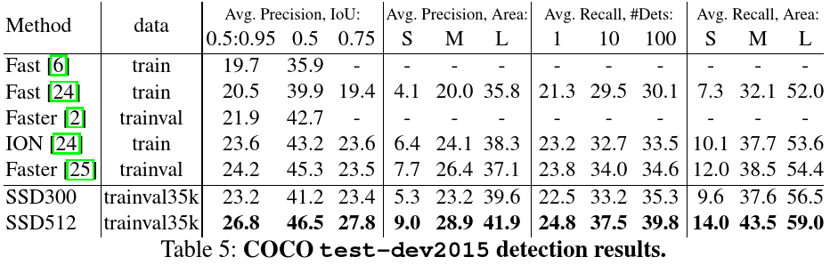
We use the trainval35k [24] for training. We first train the model with 10⁻³ learning rate for 160k iterations, and then continue training for 40k iterations with 10⁻⁴ and 40k iterations with 10⁻⁵ . Table 5 shows the results on test-dev2015. Similar to what we observed on the PASCAL VOC dataset, SSD300 is better than Fast R-CNN in both mAP@0.5 and mAP@[0.5:0.95]. SSD300 has a similar mAP@0.75 as ION [24] and Faster R-CNN [25], but is worse in mAP@0.5. By increasing the image size to 512 × 512, our SSD512 is better than Faster R-CNN [25] in both criteria. Interestingly, we observe that SSD512 is 5.3% better in mAP@0.75, but is only 1.2% better in mAP@0.5.
＃我们使用trainval35k[24]进行训练．我们首先使用10^-3的学习率训练了160k个iterations，然后继续使用10^-4的学习率训练了40k个iterations以及10^-5的学习率训练了40k个iterations.表５展示了test-dev2015数据集上的结果.结果与我们在PASCAL VOC数据集上发现的相似，SSD300在mAP@0.5和mAP@[0.5:0.95]上都超越了Fast R-CNN.SSD300在mAP@0.75上的结果与ION[24]和Faster R-CNN[25]类似，但是在mAP@0.5上结果更差．通过把图像尺寸增加到512*512，我们的SSD模型在这些准则中都超越了Faster R-CNN[25].有趣的是，我们发现SSD512在mAP@0.75上超出了5.3%，但在mAP@0.5上只超出了1.2%.
We also observe that it has much better AP (4.8%) and AR (4.6%) for large objects, but has relatively less improvement in AP (1.3%) and AR (2.0%) for small objects. Compared to ION, the improvement in AR for large and small objects is more similar (5.4% vs. 3.9%). We conjecture that Faster R-CNN is more competitive on smaller objects with SSD because it performs two box refinement steps, in both the RPN part and in the Fast R-CNN part. In Fig. 5, we show some detection examples on COCO test-dev with the SSD512 model
#同时我们也发现它(SSD)在大的物体上超出更多的平均准确率，分别为4.8%和4.6%，但是在小的物体上超出更少的平均准确率，分别为1.3%和2.0%.与ION相比，在大物体和小物体上平均准确率的改善更为接近(5.4% vs 3.9%).我们推测Faster R-CNN相比SSD在小物体(检测)上更具竞争力，因为它是通过两个box强化阶段实现的，分别为RPN和Fast R-CNN部分．在表５，我们展示了一些SSD512模型在COCO test-dev数据集的检测样本.

3.5 Preliminary ILSVRC results

We applied the same network architecture we used for COCO to the ILSVRC DET dataset [16]. We train a SSD300 model using the ILSVRC2014 DET train and val1 as used in [22]. We first train the model with 10⁻³ learning rate for 320k iterations, and then continue training for 80k iterations with 10⁻⁴ and 40k iterations with 10⁻⁵ . We can achieve 43.4 mAP on the val2 set [22]. Again, it validates that SSD is a general framework for high quality real-time detection
#我们在ILSVRC DET数据集上使用了在COCO数据集[16]上使用的相同网络结构.我们使用文献[22]中使用的ILSVRC2014 DET train和val1数据集训练SSD300模型.我们首先使用10^-3的学习率训练了320k个iterations，然后继续使用10^-4的学习率训练了80k个iterations以及10^-5的学习率训练了40k个iterations.我们可以在val2数据集上实现43.4%的平均准确率.这又一次验证了SSD是一个通用型的高质量实时检测器.

3.6 Data Augmentation for Small Object Accuracy

Without a follow-up feature resampling step as in Faster R-CNN, the classification task for small objects is relatively hard for SSD, as demonstrated in our analysis (see Fig. 4).The data augmentation strategy described in Sec. 2.2 helps to improve the performance dramatically, especially on small datasets such as PASCAL VOC. The random crops generated by the strategy can be thought of as a ”zoom in” operation and can generate many larger training examples. To implement a ”zoom out” operation that creates more small training examples, we first randomly place an image on a canvas of 16× of the original image size filled with mean values before we do any random crop operation.
#如果不沿用Faster R-CNN中使用的特征重采样步骤，对于SSD来说检测细小问题的任务尤为困难，如我们的分析中描述的一样(见图4)．Sec.2.2中描述的数据增广策略有助于极大地改善表现，尤其是在例如PASCAL VOC这样的小数据集上.(数据增广)策略中产生的随机裁剪被当作＂Zoom in(放大)＂操作，并可以产生许多更大的样本.为了通过"Zoom out(缩小)"操作产生更多细小的训练样本，在任何裁剪操作之前我们首先随机选取一张图像填充到原始图像16倍大小的画布上.
Because we have more training images by introducing this new ”expansion” data augmentation trick, we have to double the training iterations. We have seen a consistent increase of 2%-3% mAP across multiple datasets, as shown in Table 6. In specific, Figure 6 shows that the new augmentation trick significantly improves the performance on small objects. This result underscores the importance of the data augmentation strategy for the final model accuracy
#引入这个新的"扩张"数据增广方法，我们拥有更多的训练图像，我们需要将训练iterations加倍．我们发现准确率在不同数据集上拥有一致的增长(2%~3%),如表6所示．具体而言，表6展示了性的增广方法显著改善了细小物体上的(检测)性能.这个结果强调了数据增广策略对最终模型准确率的重要性.
An alternative way of improving SSD is to design a better tiling of default boxes so that its position and scale are better aligned with the receptive field of each position on a feature map. We leave this for future work
#提高SSD性能的其中一个办法是设计一个更好的default boxes　tiling方法，因此它的位置和尺寸可以更好的与特征图上每个位置的感受野相对应.我们把这个留到后续工作.

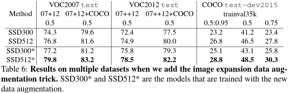
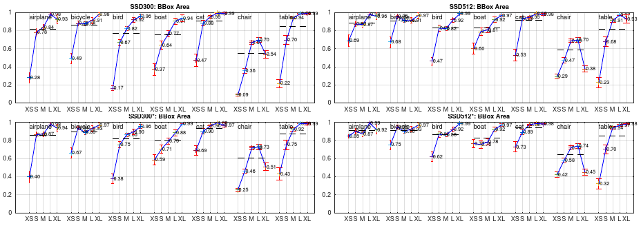
　Fig. 6: Sensitivity and impact of object size with new data augmentation on VOC2007 test set using [21]. The top row shows the effects of BBox Area per category for the original SSD300 and SSD512 model, and the bottom row corresponds to the SSD300* and SSD512* model trained with the new data augmentation trick. It is obvious that the new data augmentation trick helps detecting small objects significantly

　#在VOC2007测试数据集使用文献[21]中所述数据增广方法带来的影响．第一行展示了原始SSD300及SSD512模型中每个类别的BBox Area的影响，最后一行展示经过新的数据增广方法后的SSD300*和SSD512模型.显然新的数据增广方法很大程度上帮助检测细小物体．

3.7 Inference time

Considering the large number of boxes generated from our method, it is essential to perform non-maximum suppression (nms) efficiently during inference. By using a confidence threshold of 0.01, we can filter out most boxes. We then apply nms with jaccard overlap of 0.45 per class and keep the top 200 detections per image. This step costs about 1.7 msec per image for SSD300 and 20 VOC classes, which is close to the total time (2.4 msec) spent on all newly added layers. We measure the speed with batch size 8 using Titan X and cuDNN v4 with Intel Xeon E5-2667v3@3.20GHz
#考虑到我们的方法产生大量的boxes，有必要在推理阶段高效的运行非最大值抑制．通过把置信度阈值设置为0.01，我们可以过滤掉大多数boxes．我们随后应用jaccard overlap为0.45的非最大值抑制，并保留每张图上前200个检测.这个步骤对于SSD300上20个VOC类别来说耗费了1.7毫秒，与所有新增的网络层上消耗的时间接近．我们使用Titan X及cuDNN v4 with Intel Xeon E5-2667v3@3.20GHz进行速度测量．


Table 7: Results on Pascal VOC2007 test. SSD300 is the only real-time detection method that can achieve above 70% mAP. By using a larger input image, SSD512 outperforms all methods on accuracy while maintaining a close to real-time speed
#表７：Pascal VOC2007测试集上的结果.SSD是唯一能够实现70%以上mAP的实时检测方法．通过使用更大的输入图像，SSD512在保持近乎实时速度的同时在准确率上超越了所有方法.

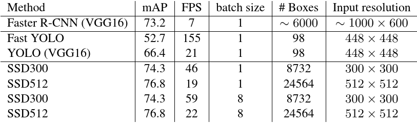
Table 7 shows the comparison between SSD, Faster R-CNN[2], and YOLO[5]. Both our SSD300 and SSD512 method outperforms Faster R-CNN in both speed and accuracy. Although Fast YOLO[5] can run at 155 FPS, it has lower accuracy by almost 22% mAP. To the best of our knowledge, SSD300 is the first real-time method to achieve above 70% mAP. Note that about 80% of the forward time is spent on the base network(VGG16 in our case). Therefore, using a faster base network could even further improve the speed, which can possibly make the SSD512 model real-time as well 
＃表7展示了SSD，Faster R-CNN[2]，YOLO[5]之间的比较.我们的SSD300和SSD512方法在速度和准确率上都超过了Faster R-CNN.虽然Fast YOLO[5]可以运行在155FPS，但是它的准确率低了接近22%.我们目前已经的知识中，SSD300是第一个平均准确率达到70%的实时检测方法．注意80%的前向时间都消耗在基础网络(本例中是VGG16).因此，使用一个更快的基础网络在未来甚至可以进一步提高运行速度，这可以使SSD512也可以达到实时应用．

Related Work

There are two established classes of methods for object detection in images, one based on sliding windows and the other based on region proposal classification. Before the advent of convolutional neural networks, the state of the art for those two approaches – Deformable Part Model (DPM) [26] and Selective Search [1] – had comparable performance. However, after the dramatic improvement brought on by R-CNN [22], which combines selective search region proposals and convolutional network based post-classification, region proposal object detection methods became prevalent
＃目前图像目标检测已经确立的方法主要有两种：一种基于sliding windows，另一种基于region proposal分类.在卷积神经网络出现之前，两种方法(DPM和Selective Proposal[1])的state-of-the-art具有可以相互比拟的表现．但是，把Selective Search region proposals与基于后分类的卷积神经网络结合在一起的R-CNN[2]带来巨大的改进之后，基于region proposal的目标检测方法开始流行
The original R-CNN approach has been improved in a variety of ways. The first set of approaches improve the quality and speed of post-classification, since it requires the classification of thousands of image crops, which is expensive and time-consuming.SPPnet [9] speeds up the original R-CNN approach significantly. It introduces a spatial pyramid pooling layer that is more robust to region size and scale and allows the classification layers to reuse features computed over feature maps generated at several image resolutions. Fast R-CNN [6] extends SPPnet so that it can fine-tune all layers end-to-end by minimizing a loss for both confidences and bounding box regression, which was first introduced in MultiBox [7] for learning objectness
＃原版R-CNN已经被不同程度地改进了．第一种方法(sliding windows)提高了后分类的质量和速度，因为它需要对数千种图像crops进行分类，这是昂贵并且费时的．SPPnet[9]很大程度上加速了原版R-CNN，它引入的空间金字塔池化层对region尺寸具有更高的鲁棒性，同时允许分类层重新使用不同图像分辨率特征图的特征．Fast R-CNN[6]在SPPnet的基础上作了进一步拓展，所以它可以基于最小化分类概率和bounding box回归的损失对所有层进行端到端fine-tune,这个最早是MultiBox[7]在学习负样本的时候引入的．
The second set of approaches improve the quality of proposal generation using deep neural networks. In the most recent works like MultiBox [7,8], the Selective Search region proposals, which are based on low-level image features, are replaced by proposals generated directly from a separate deep neural network. This further improves the detection accuracy but results in a somewhat complex setup, requiring the training of two neural networks with a dependency between them
#第二种方法通过深度神经网络来改进region proposal generation 的质量，近期大多数例如MultiBox[7,8]的作品中，所用一个独立的深度学习网络直接产生proposals替代基于低层次图像特征的Selective Search region proposals.这进一步提高了检测准确率，但是在某种程度上导致了复杂的setup,需要训练互相依赖的两个神经网络．
Faster R-CNN [2] replaces selective search proposals by ones learned from a region proposal network (RPN), and introduces a method to integrate the RPN with Fast R-CNN by alternating between fine-tuning shared convolutional layers and prediction layers for these two networks. This way region proposals are used to pool mid-level features and the final classification step is less expensive
＃Faster R-CNN[2]使用一个region proposal network[RPN]替换Selective Proposal，并引入了一种卷积层和预测层交替fine-tuning方法以实现RPN和Fast R-CNN的融合．这样region proposals被用于池化中层特征，最后的分类步骤相对不那么昂贵．
Our SSD is very similar to the region proposal network (RPN) in Faster R-CNN in that we also use a fixed set of (default) boxes for prediction, similar to the anchor boxes in the RPN. But instead of using these to pool features and evaluate another classifier, we simultaneously produce a score for each object category in each box. Thus, our approach avoids the complication of merging RPN with Fast R-CNN and is easier to train, faster, and straightforward to integrate in other tasks
＃我们的SSD与Fast R-CNN这种使用region proposal network(RPN)非常相似，我们也使用固定的一系列(default)boxes进行预测．类似于RPN中anchor boxes.但是我们同时对每个box中的每个物体进行评分，而不是将这些对特征进行池化操作并评估另外的分类器．因此，我们的方法避免了将RPN与Fast R-CNN的复杂性，因此更容易训练，运行更快，更容易集成到其他任务中去．
Another set of methods, which are directly related to our approach, skip the proposal step altogether and predict bounding boxes and confidences for multiple categories directly. OverFeat [4], a deep version of the sliding window method, predicts a bounding box directly from each location of the topmost feature map after knowing the confidences of the underlying object categories.YOLO [5] uses the whole topmost feature map to predict both confidences for multiple categories and bounding boxes (which are shared for these categories)
#另外一种方法，与我们的方法直接相关，跳过了proposal步骤，直接预测bounding boxes坐标及多个物体的评分.OverFeat[4]，一个sliding window的深度版本，在知道了潜在物体类别的置信度后直接从特征图的前几个位置预测bounding box的定位．YoLo[5]使用所有前几个特征图来预测多个类别的置信度和bounding boxes(这些类别所共享的).
Our SSD method falls in this category because we do not have the proposal step but use the default boxes. However, our approach is more flexible than the existing methods because we can use default boxes of different aspect ratios on each feature location from multiple feature maps at different scales. If we only use one default box per location from the topmost feature map, our SSD would have similar architecture to OverFeat [4]; if we use the whole topmost feature map and add a fully connected layer for predictions instead of our convolutional predictors, and do not explicitly consider multiple aspect ratios, we can approximately reproduce YOLO [5]
#我们的SSD方法属于这一类算法因为我们没有proposal步骤，但也使用了default boxes.但是我们的方法比现有的方法都更加灵活因为我们可以在多个不同尺度的每个特征点上使用不同宽高比的default boxes.如果我们在特征图前几个特征的每个位置只使用一个default box，我们的SSD结构将会与OverFeat[4]类似；如果我们使用特征图上的所有前几个特征，并且使用全连接层预测取代卷积预测，以及不明确考虑多个宽高比，我们大致可以复现YoLo[5].

Conclusion

This paper introduces SSD, a fast single-shot object detector for multiple categories. A key feature of our model is the use of multi-scale convolutional bounding box outputs attached to multiple feature maps at the top of the network. This representation allows us to efficiently model the space of possible box shapes. We experimentally validate that given appropriate training strategies, a larger number of carefully chosen default bounding boxes results in improved performance.
＃本篇文章引入了SSD，一个快速的single-shot多类别目标检测器．我们所用模型的关键特征是在网络顶端多重特征图附加多尺度卷积bounding box输出.这种表示方法允许我们高效的表征可能的box形状空间．我们的实验证实给定合适的训练类别，大量仔细挑选的default bounding boxes可以促进性能的改善
We build SSD models with at least an order of magnitude more box predictions sampling location, scale, and aspect ratio, than existing methods [5,7]. We demonstrate that given the same VGG-16 base architecture,SSD compares favorably to its state-of-the-art object detector counterparts in terms of both accuracy and speed
＃我们建立的模型与之前的方法[5,7]相比在box预测采样定位，尺度，宽度至少高一个数量级．我们展示了使用相同的VGG-16基础结构，SSD在准确率和速度上都轻松超越之前的state-of-the-art目标检测器．
Our SSD512 model significantly outperforms the state-of-the-art Faster R-CNN [2] in terms of accuracy on PASCAL VOC and COCO, while being 3× faster. Our real time SSD300 model runs at 59 FPS, which is faster than the current real time YOLO [5] alternative, while producing markedly superior detection accuracy
＃我们的SSD512模型在PASCAL VOC及COCO数据集上的准确率明显超越了state-of-the-art Faster R-CNN[2],同时保持3倍更快的速度．我们的实时SSD300以59FPS速度运行，相当当前的实时YoLo[5]更快，同时拥有显著优化的检测准确率．
Apart from its standalone utility, we believe that our monolithic and relatively simple SSD model provides a useful building block for larger systems that employ an object detection component. A promising future direction is to explore its use as part of a system using recurrent neural networks to detect and track objects in video simultaneously
＃除了它单独的用途，我们相信整体及相对简单的SSD模型为更大目标检测系统提供有价值的基石．一个非常有前景的发展方向是探索把它作为即时视频应用中循环神经网络进行探测跟踪的一部分.

　　　　参考文献

　　　　1.https://blog.csdn.net/u014380165/article/details/72824889