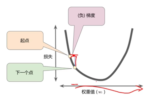
总是朝着负梯度的方向进行下一步探索
梯度乘学习率 = 权重值的下一个位置
超参数:在学习开始过程之前设置的参数
在jupyter中,用matplotlib显示图像需设置为inline模式,必须加上一行
%matplotlib inline
np.random.rand(d0,d1,d2……dn)   #有几个数表示几维,且在此维的长度是多少
注:使用方法与np.random.randn()函数相同
作用:
通过本函数可以返回一个或一组服从“0~1”均匀分布的随机样本值。随机样本取值范围是[0,1),不包括1。


设x_data为一个一维数组
x_data.shape的输出为(100,)
*x_data.shape的输出为100
#tensorflow的变量,tf.Variable用于保存和更新参数,初值可任意
w = tf.Variable(1.0, tf.float32)
b = tf.Variable(0.0, tf.float32)
优化器,就是tensorflow中梯度下降的策略,用于更新神经网络中数以百万的参数。
tensorflow2.0中使用梯度带的形式,定义一个gradient函数使用
def grad(x, y, w, b):
    with tf.GradientTape as tape:
        loss_ = loss(x1, y1, w, b)
    return tape.gradient(loss_, [w, b]) #其中[]中的参数有几个,则返回值就有几个,每个返回值即为对应参数的梯度
#用梯度 * 学习率即为每个参数需要调整的值
w_step, b_step = grad(x, y, w, b)
w.assgin_sub(w_step * learn_rate) #梯度为负数,因此为sub
b.assign_sun(b_step * learn_rate)
code:


%matplotlib inline
import tensorflow as tf
import numpy as np
from matplotlib import pyplot as plt

x_data = np.linspace(-1, 1, 100)
y_data = x_data * 2.0 + 1.0 + np.random.randn(100) * 0.4

w = tf.Variable(initial_value = 1.0)
b = tf.Variable(initial_value = 0.0)

def cul(x, w, b):
    return x * w + b

def loss_f(x, y, w, b):
    return tf.reduce_mean(tf.square(y - cul(x, w, b)))

def grad(x, y, w, b):
    with tf.GradientTape() as tap:
        loss_ = loss_f(x, y, w, b)
    return tap.gradient(loss_, [w, b])

learn_rate = 0.01

for i in range(100):
    loss_ = loss_f(x_data, y_data, w, b)
    w_step, b_step = grad(x_data, y_data, w, b)
    w.assign_sub(w_step * learn_rate)
    b.assign_sub(b_step * learn_rate)
    print("Train: %d, Loss = %f" %(i + 1, loss_))


plt.scatter(x_data, y_data)

plt.plot(x_data, x_data * w + b)