里程碑式创新:ResNet
2015年何恺明推出的ResNet在ISLVRC和COCO上横扫所有选手,获得冠军。ResNet在网络结构上做了大创新,而不再是简单的堆积层数,ResNet在卷积神经网络的新思路,绝对是深度学习发展历程上里程碑式的事件。

闪光点:
- 层数非常深,已经超过百层
- 引入残差单元来解决退化问题
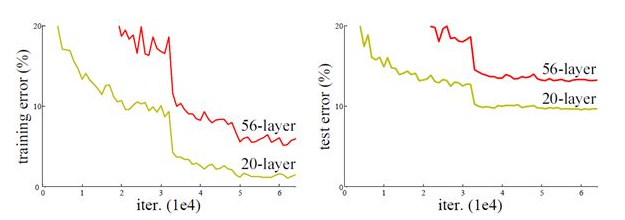
从前面可以看到,随着网络深度增加,网络的准确度应该同步增加,当然要注意过拟合问题。但是网络深度增加的一个问题在于这些增加的层是参数更新的信号,因为梯度是从后向前传播的,增加网络深度后,比较靠前的层梯度会很小。这意味着这些层基本上学习停滞了,这就是梯度消失问题。深度网络的第二个问题在于训练,当网络更深时意味着参数空间更大,优化问题变得更难,因此简单地去增加网络深度反而出现更高的训练误差,深层网络虽然收敛了,但网络却开始退化了,即增加网络层数却导致更大的误差,比如下图,一个56层的网络的性能却不如20层的性能好,这不是因为过拟合(训练集训练误差依然很高),这就是烦人的退化问题。残差网络ResNet设计一种残差模块让我们可以训练更深的网络。
这里详细分析一下残差单元来理解ResNet的精髓。
从下图可以看出,数据经过了两条路线,一条是常规路线,另一条则是捷径(shortcut),直接实现单位映射的直接连接的路线,这有点类似与电路中的“短路”。通过实验,这种带有shortcut的结构确实可以很好地应对退化问题。我们把网络中的一个模块的输入和输出关系看作是y=H(x),那么直接通过梯度方法求H(x)就会遇到上面提到的退化问题,如果使用了这种带shortcut的结构,那么可变参数部分的优化目标就不再是H(x),若用F(x)来代表需要优化的部分的话,则H(x)=F(x)+x,也就是F(x)=H(x)-x。因为在单位映射的假设中y=x就相当于观测值,所以F(x)就对应着残差,因而叫残差网络。为啥要这样做,因为作者认为学习残差F(X)比直接学习H(X)简单!设想下,现在根据我们只需要去学习输入和输出的差值就可以了,绝对量变为相对量(H(x)-x 就是输出相对于输入变化了多少),优化起来简单很多。
考虑到x的维度与F(X)维度可能不匹配情况,需进行维度匹配。这里论文中采用两种方法解决这一问题(其实是三种,但通过实验发现第三种方法会使performance急剧下降,故不采用):
- zero_padding:对恒等层进行0填充的方式将维度补充完整。这种方法不会增加额外的参数
- projection:在恒等层采用1x1的卷积核来增加维度。这种方法会增加额外的参数

下图展示了两种形态的残差模块,左图是常规残差模块,有两个3×3卷积核卷积核组成,但是随着网络进一步加深,这种残差结构在实践中并不是十分有效。针对这问题,右图的“瓶颈残差模块”(bottleneck residual block)可以有更好的效果,它依次由1×1、3×3、1×1这三个卷积层堆积而成,这里的1×1的卷积能够起降维或升维的作用,从而令3×3的卷积可以在相对较低维度的输入上进行,以达到提高计算效率的目的。

ResNet-50的Keras实现:
def Conv2d_BN(x, nb_filter,kernel_size, strides=(1,1), padding='same',name=None):
    if name is not None:
        bn_name = name + '_bn'
        conv_name = name + '_conv'
    else:
        bn_name = None
        conv_name = None

    x = Conv2D(nb_filter,kernel_size,padding=padding,strides=strides,activation='relu',name=conv_name)(x)
    x = BatchNormalization(axis=3,name=bn_name)(x)
    return x

def Conv_Block(inpt,nb_filter,kernel_size,strides=(1,1), with_conv_shortcut=False):
    x = Conv2d_BN(inpt,nb_filter=nb_filter[0],kernel_size=(1,1),strides=strides,padding='same')
    x = Conv2d_BN(x, nb_filter=nb_filter[1], kernel_size=(3,3), padding='same')
    x = Conv2d_BN(x, nb_filter=nb_filter[2], kernel_size=(1,1), padding='same')
    if with_conv_shortcut:
        shortcut = Conv2d_BN(inpt,nb_filter=nb_filter[2],strides=strides,kernel_size=kernel_size)
        x = add([x,shortcut])
        return x
    else:
        x = add([x,inpt])
        return x

def ResNet50():
    inpt = Input(shape=(224,224,3))
    x = ZeroPadding2D((3,3))(inpt)
    x = Conv2d_BN(x,nb_filter=64,kernel_size=(7,7),strides=(2,2),padding='valid')
    x = MaxPooling2D(pool_size=(3,3),strides=(2,2),padding='same')(x)

    x = Conv_Block(x,nb_filter=[64,64,256],kernel_size=(3,3),strides=(1,1),with_conv_shortcut=True)
    x = Conv_Block(x,nb_filter=[64,64,256],kernel_size=(3,3))
    x = Conv_Block(x,nb_filter=[64,64,256],kernel_size=(3,3))

    x = Conv_Block(x,nb_filter=[128,128,512],kernel_size=(3,3),strides=(2,2),with_conv_shortcut=True)
    x = Conv_Block(x,nb_filter=[128,128,512],kernel_size=(3,3))
    x = Conv_Block(x,nb_filter=[128,128,512],kernel_size=(3,3))
    x = Conv_Block(x,nb_filter=[128,128,512],kernel_size=(3,3))

    x = Conv_Block(x,nb_filter=[256,256,1024],kernel_size=(3,3),strides=(2,2),with_conv_shortcut=True)
    x = Conv_Block(x,nb_filter=[256,256,1024],kernel_size=(3,3))
    x = Conv_Block(x,nb_filter=[256,256,1024],kernel_size=(3,3))
    x = Conv_Block(x,nb_filter=[256,256,1024],kernel_size=(3,3))
    x = Conv_Block(x,nb_filter=[256,256,1024],kernel_size=(3,3))
    x = Conv_Block(x,nb_filter=[256,256,1024],kernel_size=(3,3))

    x = Conv_Block(x,nb_filter=[512,512,2048],kernel_size=(3,3),strides=(2,2),with_conv_shortcut=True)
    x = Conv_Block(x,nb_filter=[512,512,2048],kernel_size=(3,3))
    x = Conv_Block(x,nb_filter=[512,512,2048],kernel_size=(3,3))
    x = AveragePooling2D(pool_size=(7,7))(x)
    x = Flatten()(x)
    x = Dense(1000,activation='softmax')(x)

    model = Model(inputs=inpt,outputs=x)
    return model
继往开来:DenseNet
自Resnet提出以后,ResNet的变种网络层出不穷,都各有其特点,网络性能也有一定的提升。本文介绍的最后一个网络是CVPR 2017最佳论文DenseNet,论文中提出的DenseNet(Dense Convolutional Network)主要还是和ResNet及Inception网络做对比,思想上有借鉴,但却是全新的结构,网络结构并不复杂,却非常有效,在CIFAR指标上全面超越ResNet。可以说DenseNet吸收了ResNet最精华的部分,并在此上做了更加创新的工作,使得网络性能进一步提升。
闪光点:
- 密集连接:缓解梯度消失问题,加强特征传播,鼓励特征复用,极大的减少了参数量
DenseNet 是一种具有密集连接的卷积神经网络。在该网络中,任何两层之间都有直接的连接,也就是说,网络每一层的输入都是前面所有层输出的并集,而该层所学习的特征图也会被直接传给其后面所有层作为输入。下图是 DenseNet 的一个dense block示意图,一个block里面的结构如下,与ResNet中的BottleNeck基本一致:BN-ReLU-Conv(1×1)-BN-ReLU-Conv(3×3) ,而一个DenseNet则由多个这种block组成。每个DenseBlock的之间层称为transition layers,由BN−>Conv(1×1)−>averagePooling(2×2)组成

密集连接不会带来冗余吗?不会!密集连接这个词给人的第一感觉就是极大的增加了网络的参数量和计算量。但实际上 DenseNet 比其他网络效率更高,其关键就在于网络每层计算量的减少以及特征的重复利用。DenseNet则是让l层的输入直接影响到之后的所有层,它的输出为:xl=Hl([X0,X1,…,xl−1]),其中[x0,x1,...,xl−1]就是将之前的feature map以通道的维度进行合并。并且由于每一层都包含之前所有层的输出信息,因此其只需要很少的特征图就够了,这也是为什么DneseNet的参数量较其他模型大大减少的原因。这种dense connection相当于每一层都直接连接input和loss,因此就可以减轻梯度消失现象,这样更深网络不是问题
需要明确一点,dense connectivity 仅仅是在一个dense block里的,不同dense block 之间是没有dense connectivity的,比如下图所示。

综合来看,DenseNet的优势主要体现在以下几个方面:
- 由于密集连接方式,DenseNet提升了梯度的反向传播,使得网络更容易训练。由于每层可以直达最后的误差信号,实现了隐式的“deep supervision”;
- 参数更小且计算更高效,这有点违反直觉,由于DenseNet是通过concat特征来实现短路连接,实现了特征重用,并且采用较小的growth rate,每个层所独有的特征图是比较小的;
- 由于特征复用,最后的分类器使用了低级特征。
天底下没有免费的午餐,网络自然也不例外。在同层深度下获得更好的收敛率,自然是有额外代价的。其代价之一,就是其恐怖如斯的内存占用。
DenseNet-121的Keras实现:
def DenseNet121(nb_dense_block=4, growth_rate=32, nb_filter=64, reduction=0.0, dropout_rate=0.0, weight_decay=1e-4, classes=1000, weights_path=None):
    '''Instantiate the DenseNet 121 architecture,
        # Arguments
            nb_dense_block: number of dense blocks to add to end
            growth_rate: number of filters to add per dense block
            nb_filter: initial number of filters
            reduction: reduction factor of transition blocks.
            dropout_rate: dropout rate
            weight_decay: weight decay factor
            classes: optional number of classes to classify images
            weights_path: path to pre-trained weights
        # Returns
            A Keras model instance.
    '''
    eps = 1.1e-5

    # compute compression factor
    compression = 1.0 - reduction

    # Handle Dimension Ordering for different backends
    global concat_axis
    if K.image_dim_ordering() == 'tf':
      concat_axis = 3
      img_input = Input(shape=(224, 224, 3), name='data')
    else:
      concat_axis = 1
      img_input = Input(shape=(3, 224, 224), name='data')

    # From architecture for ImageNet (Table 1 in the paper)
    nb_filter = 64
    nb_layers = [6,12,24,16] # For DenseNet-121

    # Initial convolution
    x = ZeroPadding2D((3, 3), name='conv1_zeropadding')(img_input)
    x = Convolution2D(nb_filter, 7, 7, subsample=(2, 2), name='conv1', bias=False)(x)
    x = BatchNormalization(epsilon=eps, axis=concat_axis, name='conv1_bn')(x)
    x = Scale(axis=concat_axis, name='conv1_scale')(x)
    x = Activation('relu', name='relu1')(x)
    x = ZeroPadding2D((1, 1), name='pool1_zeropadding')(x)
    x = MaxPooling2D((3, 3), strides=(2, 2), name='pool1')(x)

    # Add dense blocks
    for block_idx in range(nb_dense_block - 1):
        stage = block_idx+2
        x, nb_filter = dense_block(x, stage, nb_layers[block_idx], nb_filter, growth_rate, dropout_rate=dropout_rate, weight_decay=weight_decay)

        # Add transition_block
        x = transition_block(x, stage, nb_filter, compression=compression, dropout_rate=dropout_rate, weight_decay=weight_decay)
        nb_filter = int(nb_filter * compression)

    final_stage = stage + 1
    x, nb_filter = dense_block(x, final_stage, nb_layers[-1], nb_filter, growth_rate, dropout_rate=dropout_rate, weight_decay=weight_decay)

    x = BatchNormalization(epsilon=eps, axis=concat_axis, name='conv'+str(final_stage)+'_blk_bn')(x)
    x = Scale(axis=concat_axis, name='conv'+str(final_stage)+'_blk_scale')(x)
    x = Activation('relu', name='relu'+str(final_stage)+'_blk')(x)
    x = GlobalAveragePooling2D(name='pool'+str(final_stage))(x)

    x = Dense(classes, name='fc6')(x)
    x = Activation('softmax', name='prob')(x)

    model = Model(img_input, x, name='densenet')

    if weights_path is not None:
      model.load_weights(weights_path)

    return model


def conv_block(x, stage, branch, nb_filter, dropout_rate=None, weight_decay=1e-4):
    '''Apply BatchNorm, Relu, bottleneck 1x1 Conv2D, 3x3 Conv2D, and option dropout
        # Arguments
            x: input tensor
            stage: index for dense block
            branch: layer index within each dense block
            nb_filter: number of filters
            dropout_rate: dropout rate
            weight_decay: weight decay factor
    '''
    eps = 1.1e-5
    conv_name_base = 'conv' + str(stage) + '_' + str(branch)
    relu_name_base = 'relu' + str(stage) + '_' + str(branch)

    # 1x1 Convolution (Bottleneck layer)
    inter_channel = nb_filter * 4
    x = BatchNormalization(epsilon=eps, axis=concat_axis, name=conv_name_base+'_x1_bn')(x)
    x = Scale(axis=concat_axis, name=conv_name_base+'_x1_scale')(x)
    x = Activation('relu', name=relu_name_base+'_x1')(x)
    x = Convolution2D(inter_channel, 1, 1, name=conv_name_base+'_x1', bias=False)(x)

    if dropout_rate:
        x = Dropout(dropout_rate)(x)

    # 3x3 Convolution
    x = BatchNormalization(epsilon=eps, axis=concat_axis, name=conv_name_base+'_x2_bn')(x)
    x = Scale(axis=concat_axis, name=conv_name_base+'_x2_scale')(x)
    x = Activation('relu', name=relu_name_base+'_x2')(x)
    x = ZeroPadding2D((1, 1), name=conv_name_base+'_x2_zeropadding')(x)
    x = Convolution2D(nb_filter, 3, 3, name=conv_name_base+'_x2', bias=False)(x)

    if dropout_rate:
        x = Dropout(dropout_rate)(x)

    return x


def transition_block(x, stage, nb_filter, compression=1.0, dropout_rate=None, weight_decay=1E-4):
    ''' Apply BatchNorm, 1x1 Convolution, averagePooling, optional compression, dropout
        # Arguments
            x: input tensor
            stage: index for dense block
            nb_filter: number of filters
            compression: calculated as 1 - reduction. Reduces the number of feature maps in the transition block.
            dropout_rate: dropout rate
            weight_decay: weight decay factor
    '''

    eps = 1.1e-5
    conv_name_base = 'conv' + str(stage) + '_blk'
    relu_name_base = 'relu' + str(stage) + '_blk'
    pool_name_base = 'pool' + str(stage)

    x = BatchNormalization(epsilon=eps, axis=concat_axis, name=conv_name_base+'_bn')(x)
    x = Scale(axis=concat_axis, name=conv_name_base+'_scale')(x)
    x = Activation('relu', name=relu_name_base)(x)
    x = Convolution2D(int(nb_filter * compression), 1, 1, name=conv_name_base, bias=False)(x)

    if dropout_rate:
        x = Dropout(dropout_rate)(x)

    x = AveragePooling2D((2, 2), strides=(2, 2), name=pool_name_base)(x)

    return x


def dense_block(x, stage, nb_layers, nb_filter, growth_rate, dropout_rate=None, weight_decay=1e-4, grow_nb_filters=True):
    ''' Build a dense_block where the output of each conv_block is fed to subsequent ones
        # Arguments
            x: input tensor
            stage: index for dense block
            nb_layers: the number of layers of conv_block to append to the model.
            nb_filter: number of filters
            growth_rate: growth rate
            dropout_rate: dropout rate
            weight_decay: weight decay factor
            grow_nb_filters: flag to decide to allow number of filters to grow
    '''

    eps = 1.1e-5
    concat_feat = x

    for i in range(nb_layers):
        branch = i+1
        x = conv_block(concat_feat, stage, branch, growth_rate, dropout_rate, weight_decay)
        concat_feat = merge([concat_feat, x], mode='concat', concat_axis=concat_axis, name='concat_'+str(stage)+'_'+str(branch))

        if grow_nb_filters:
            nb_filter += growth_rate

    return concat_feat, nb_filter
转自:https://www.cnblogs.com/skyfsm/p/8451834.html