霍夫变换

在图片处理中，霍夫变换主要是用来检测图片中的几何形状，包括直线、圆、椭圆等。在skimage中，霍夫变换是放在tranform模块内。

一 霍夫线变换

 对于平面中的一条直线，在笛卡尔坐标系中，可用y=mx+b来表示，其中m为斜率，b为截距。但是如果直线是一条垂直线，则m为无穷大，所有通常我们在另一坐标系中表示直线，即极坐标系下的r=xcos(theta)+ysin(theta)。即可用（r,theta）来表示一条直线。其中r为该直线到原点的距离，theta为该直线的垂线与x轴的夹角。如下图所示。

对于一个给定的点（x0,y0), 我们在极坐标下绘出所有通过它的直线（r,theta)，将得到一条正弦曲线。如果将图片中的所有非0点的正弦曲线都绘制出来，则会存在一些交点。所有经过这个交点的正弦曲线，说明都拥有同样的(r,theta), 意味着这些点在一条直线上。

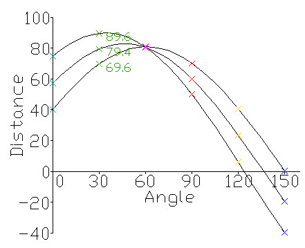
如上图所示，三个点(对应图中的三条正弦曲线）在一条直线上，因为这三个曲线交于一点，具有相同的（r, theta)。霍夫线变换就是利用这种方法来寻找图中的直线。

函数：skimage.transform.hough_line(img)

返回三个值：

• h: 霍夫变换累积器
• theta: 点与x轴的夹角集合，一般为0-179度
• distance: 点到原点的距离，即上面的所说的r.

import skimage.transform as st
import numpy as np
import matplotlib.pyplot as plt

# 构建测试图片
image = np.zeros((100, 100))  #背景图
idx = np.arange(25, 75)    #25-74序列
image[idx[::-1], idx] = 255  # 线条
image[idx, idx] = 255        # 线条/

# hough线变换
h, theta, d = st.hough_line(image)

#生成一个一行两列的窗口（可显示两张图片）.
fig, (ax0, ax1) = plt.subplots(1, 2, figsize=(8, 6))
plt.tight_layout()

#显示原始图片
ax0.imshow(image, plt.cm.gray)
ax0.set_title('Input image')
ax0.set_axis_off()

#显示hough变换所得数据
ax1.imshow(np.log(1 + h))
ax1.set_title('Hough transform')
ax1.set_xlabel('Angles (degrees)')
ax1.set_ylabel('Distance (pixels)')
ax1.axis('image')

结果如下图所示：

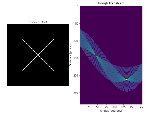
从右边那张图可以看出，有两个交点，说明原图像中有两条直线。如果我们要把图中的两条直线绘制出来，则需要用到另外一个函数：

                skimage.transform.hough_line_peaks(hspace, angles, dists）

用这个函数可以取出峰值点，即交点，也即原图中的直线。返回的参数与输入的参数一样。我们修改一下上边的程序，在原图中将两直线绘制出来。

import skimage.transform as st
import numpy as np
import matplotlib.pyplot as plt

# 构建测试图片
image = np.zeros((100, 100))  #背景图
idx = np.arange(25, 75)    #25-74序列
image[idx[::-1], idx] = 255  # 线条
image[idx, idx] = 255        # 线条/

# hough线变换
h, theta, d = st.hough_line(image)

#生成一个一行三列的窗口（可显示三张图片）.
fig, (ax0, ax1,ax2) = plt.subplots(1, 3, figsize=(8, 6))
plt.tight_layout()

#显示原始图片
ax0.imshow(image, plt.cm.gray)
ax0.set_title('Input image')
ax0.set_axis_off()

#显示hough变换所得数据
ax1.imshow(np.log(1 + h))
ax1.set_title('Hough transform')
ax1.set_xlabel('Angles (degrees)')
ax1.set_ylabel('Distance (pixels)')
ax1.axis('image')

#显示检测出的线条
ax2.imshow(image, plt.cm.gray)
row1, col1 = image.shape
for _, angle, dist in zip(*st.hough_line_peaks(h, theta, d)):
    y0 = (dist - 0 * np.cos(angle)) / np.sin(angle)
    y1 = (dist - col1 * np.cos(angle)) / np.sin(angle)
    ax2.plot((0, col1), (y0, y1), '-r')
ax2.axis((0, col1, row1, 0))
ax2.set_title('Detected lines')
ax2.set_axis_off()

结果如下图所示：

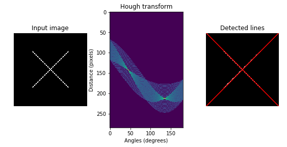
注意，绘制线条的时候，要从极坐标转换为笛卡尔坐标，公式为：

skimage还提供了另外一个检测直线的霍夫变换函数，概率霍夫线变换：

skimage.transform.probabilistic_hough_line(img, threshold=10, line_length=5,line_gap=3)

参数：

• img: 待检测的图像。
• threshold： 阈值，可先项，默认为10
• line_length: 检测的最短线条长度，默认为5
• line_gap: 线条间的最大间隙。增大这个值可以合并破碎的线条。默认为3

返回：

• lines: 线条列表, 格式如((x0, y0), (x1, y0))，标明开始点和结束点。

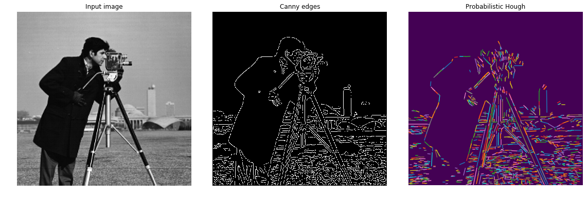
下面，我们用canny算子提取边缘，然后检测哪些边缘是直线？

import skimage.transform as st
import matplotlib.pyplot as plt
from skimage import data,feature,color

#使用Probabilistic Hough Transform.
image = data.camera()
edges = feature.canny(image, sigma=2, low_threshold=1, high_threshold=25)
lines = st.probabilistic_hough_line(edges, threshold=10, line_length=5,line_gap=3)

# 创建显示窗口.
fig, (ax0, ax1, ax2) = plt.subplots(1, 3, figsize=(16, 6))
plt.tight_layout()

#显示原图像
ax0.imshow(image, plt.cm.gray)
ax0.set_title('Input image')
ax0.set_axis_off()

#显示canny边缘
ax1.imshow(edges, plt.cm.gray)
ax1.set_title('Canny edges')
ax1.set_axis_off()

#用plot绘制出所有的直线
ax2.imshow(edges * 0)
for line in lines:
    p0, p1 = line
    ax2.plot((p0[0], p1[0]), (p0[1], p1[1]))
row2, col2 = image.shape
ax2.axis((0, col2, row2, 0))
ax2.set_title('Probabilistic Hough')
ax2.set_axis_off()
plt.show()

 结果如下图所示：

二 霍夫圆和椭圆变换

在极坐标中，圆的表示方式为：

• x=x0+rcosθ
• y=y0+rsinθ

圆心为(x0,y0),r为半径，θ为旋转度数，值范围为0-359

如果给定圆心点和半径，则其它点是否在圆上，我们就能检测出来了。在图像中，我们将每个非0像素点作为圆心点，以一定的半径进行检测，如果有一个点在圆上，我们就对这个圆心累加一次。如果检测到一个圆，那么这个圆心点就累加到最大，成为峰值。因此，在检测结果中，一个峰值点，就对应一个圆心点。

霍夫圆检测的函数：

             skimage.transform.hough_circle(image, radius)

• radius是一个数组，表示半径的集合，如[3，4，5，6]
• 返回一个3维的数组（radius index, M, N), 第一维表示半径的索引，后面两维表示图像的尺寸。

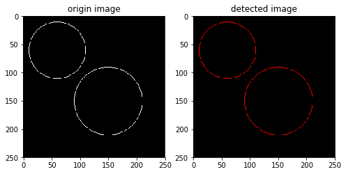
例1：绘制两个圆形，用霍夫圆变换将它们检测出来。

import numpy as np
import matplotlib.pyplot as plt
from skimage import draw,transform,feature

img = np.zeros((250, 250,3), dtype=np.uint8)
rr, cc = draw.circle_perimeter(60, 60, 50)  #以圆心为（60,60）半径为50画一个圆,
rr1, cc1 = draw.circle_perimeter(150, 150, 60) #以圆心为（150,150）半径为60画一个圆
img[cc, rr,:] =255
img[cc1, rr1,:] =255

fig, (ax0,ax1) = plt.subplots(1,2, figsize=(8, 5))

ax0.imshow(img)  #显示原图
ax0.set_title('origin image')

hough_radii = np.arange(50, 80, 5)  #半径范围
hough_res =transform.hough_circle(img[:,:,0], hough_radii)  #圆变换 

centers = []  #保存所有圆心点坐标
accums = []   #累积值
radii = []    #半径

for radius, h in zip(hough_radii, hough_res):
    #每一个半径值，取出其中两个圆
    #zip()的用法
    num_peaks = 2
    peaks =feature.peak_local_max(h, num_peaks=num_peaks) #取出峰值
    centers.extend(peaks)
    accums.extend(h[peaks[:, 0], peaks[:, 1]])
    radii.extend([radius] * num_peaks)

#画出最接近的圆
image =np.copy(img)
for idx in np.argsort(accums)[::-1][:2]:#argsort()函数是将x中的元素从小到大排列，提取其对应的index(索引)，然后输出到y
    center_x, center_y = centers[idx]
    radius = radii[idx]
    cx, cy =draw.circle_perimeter(center_y, center_x, radius)
    image[cy, cx] =(255,0,0)

ax1.imshow(image)
ax1.set_title('detected image')

结果如下图所示：

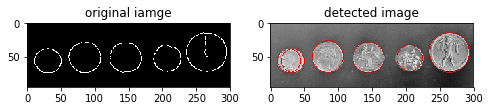
例2，检测出下图中存在的硬币。

 

import numpy as np
import matplotlib.pyplot as plt
from skimage import data, color,draw,transform,feature,util

image = util.img_as_ubyte(data.coins()[0:95, 70:370]) #裁剪原图片
edges =feature.canny(image, sigma=3, low_threshold=10, high_threshold=50) #检测canny边缘

fig, (ax0,ax1) = plt.subplots(1,2, figsize=(8, 5))

ax0.imshow(edges, cmap=plt.cm.gray)  #显示canny边缘
ax0.set_title('original iamge')

hough_radii = np.arange(15, 30, 2)  #半径范围
hough_res =transform.hough_circle(edges, hough_radii)  #圆变换 

centers = []  #保存中心点坐标
accums = []   #累积值
radii = []    #半径

for radius, h in zip(hough_radii, hough_res):
    #每一个半径值，取出其中两个圆
    num_peaks = 2
    peaks =feature.peak_local_max(h, num_peaks=num_peaks) #取出峰值
    centers.extend(peaks)
    accums.extend(h[peaks[:, 0], peaks[:, 1]])
    radii.extend([radius] * num_peaks)

#画出最接近的5个圆
image = color.gray2rgb(image)
for idx in np.argsort(accums)[::-1][:5]:
    center_x, center_y = centers[idx]
    radius = radii[idx]
    cx, cy =draw.circle_perimeter(center_y, center_x, radius)
    image[cy, cx] = (255,0,0)

ax1.imshow(image)
ax1.set_title('detected image')

结果如下图所示：

椭圆变换是类似的，使用函数为：

           skimage.transform.hough_ellipse(img,accuracy, threshold, min_size, max_size)

输入参数：

• img: 待检测图像。
• accuracy: 使用在累加器上的短轴二进制尺寸，是一个double型的值，默认为1
• thresh: 累加器阈值，默认为4
• min_size: 长轴最小长度，默认为4
• max_size: 短轴最大长度，默认为None,表示图片最短边的一半。

返回一个 [(accumulator, y0, x0, a, b, orientation)] 数组。

• accumulator表示累加器
• （y0,x0)表示椭圆中心点
• （a,b)分别表示长短轴，orientation表示椭圆方向

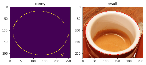
例：检测出咖啡图片中的椭圆杯口。

import matplotlib.pyplot as plt
from skimage import data,draw,color,transform,feature

#加载图片，转换成灰度图并检测边缘
image_rgb = data.coffee()[0:220, 160:420] #裁剪原图像，不然速度非常慢
image_gray = color.rgb2gray(image_rgb)
edges = feature.canny(image_gray, sigma=2.0, low_threshold=0.55, high_threshold=0.8)

#执行椭圆变换
result =transform.hough_ellipse(edges, accuracy=20, threshold=250,min_size=100, max_size=120)
result.sort(order='accumulator') #根据累加器排序

#估计椭圆参数
best = list(result[-1])  #排完序后取最后一个
yc, xc, a, b = [int(round(x)) for x in best[1:5]]
orientation = best[5]

#在原图上画出椭圆
cy, cx =draw.ellipse_perimeter(yc, xc, a, b, orientation)
image_rgb[cy, cx,:] = (255, 0, 0) #在原图中用蓝色表示检测出的椭圆

fig2, (ax1, ax2) = plt.subplots(ncols=2, nrows=1, figsize=(8, 4))

ax1.set_title('canny')
ax1.imshow(edges)

ax2.set_title('result')
ax2.imshow(image_rgb)

plt.show()

结果如下图所示：

霍夫椭圆变换速度非常慢，应避免图像太大。