定义:
支持向量机SVM(Support vector machine)是一种二值分类器方法,其基本是思想是:找到一个能够将两类分开的线性可分的直线(或者超平面)。实际上有许多条直线(或超平面)可以将两类目标分开来,我们要找的其实是这些直线(或超平面)中分割两类目标时,有最大距离的直线(或超平面)。我们称这样的直线或超平面为最佳线性分类器。如下图:

源码如下:
#引入库
import matplotlib.pyplot as plt
import numpy as np
import tensorflow as tf
from sklearn import datasets
from tensorflow.python.framework import ops
#创建图
sess = tf.Session()
#加载数据
iris = datasets.load_iris()
x_vals = np.array([[x[0], x[3]] for x in iris.data])
y_vals = np.array([1 if y == 0 else -1 for y in iris.target])
#分割数据集,80%的数据作为训练集用来训练,剩下20%的数据作为测试集用来做测试
train_indices = np.random.choice(len(x_vals),
                                 round(len(x_vals)*0.8),
                                 replace=False)
test_indices = np.array(list(set(range(len(x_vals))) - set(train_indices)))
x_vals_train = x_vals[train_indices]
x_vals_test = x_vals[test_indices]
y_vals_train = y_vals[train_indices]
y_vals_test = y_vals[test_indices]
# 声明批量大小
batch_size = 100
# 初始化占位符
x_data = tf.placeholder(shape=[None, 2], dtype=tf.float32)
y_target = tf.placeholder(shape=[None, 1], dtype=tf.float32)
# 创建变量
A = tf.Variable(tf.random_normal(shape=[2, 1]))
b = tf.Variable(tf.random_normal(shape=[1, 1]))
# 构建模型
model_output = tf.subtract(tf.matmul(x_data, A), b)
# 采用L2正则式
l2_norm = tf.reduce_sum(tf.square(A))
# 声明alpha参数
alpha = tf.constant([0.01])
term1=tf.subtract(1., tf.multiply(model_output, y_target))
classification_term = tf.reduce_mean(tf.maximum(0., term1))
# 定义损失函数
loss = tf.add(classification_term, tf.multiply(alpha, l2_norm))
# 声明预测函数和准确度函数
prediction = tf.sign(model_output)
accuracy = tf.reduce_mean(tf.cast(tf.equal(prediction, y_target), tf.float32))
# 声明优化器
my_opt = tf.train.GradientDescentOptimizer(0.01)
train_step = my_opt.minimize(loss)
# 初始化变量
init = tf.global_variables_initializer()
sess.run(init)
#迭代训练
loss_vec = []
train_accuracy = []
test_accuracy = []
for i in range(1000):
    rand_index = np.random.choice(len(x_vals_train), size=batch_size)
    rand_x = x_vals_train[rand_index]
    rand_y = np.transpose([y_vals_train[rand_index]])
    sess.run(train_step, feed_dict={x_data: rand_x, y_target: rand_y})

    temp_loss = sess.run(loss, feed_dict={x_data: rand_x, y_target: rand_y})
    loss_vec.append(temp_loss)

    train_acc_temp = sess.run(accuracy, feed_dict={
        x_data: x_vals_train,
        y_target: np.transpose([y_vals_train])})
    train_accuracy.append(train_acc_temp)

    test_acc_temp = sess.run(accuracy, feed_dict={
        x_data: x_vals_test,
        y_target: np.transpose([y_vals_test])})
    test_accuracy.append(test_acc_temp)

# 抽取系数和截距
[[a1], [a2]] = sess.run(A)
[[b]] = sess.run(b)
slope = -a2/a1
y_intercept = b/a1

x1_vals = [d[1] for d in x_vals]

#
best_fit = []
for i in x1_vals:
    best_fit.append(slope*i+y_intercept)

setosa_x = [d[1] for i, d in enumerate(x_vals) if y_vals[i] == 1]
setosa_y = [d[0] for i, d in enumerate(x_vals) if y_vals[i] == 1]
not_setosa_x = [d[1] for i, d in enumerate(x_vals) if y_vals[i] == -1]
not_setosa_y = [d[0] for i, d in enumerate(x_vals) if y_vals[i] == -1]
%matplotlib inline
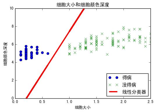
# 展示分类结果
plt.plot(setosa_x, setosa_y, 'o', label='得病')
plt.plot(not_setosa_x, not_setosa_y, 'x', label='没得病')
plt.plot(x1_vals, best_fit, 'r-', label='线性分类器', linewidth=3)
plt.ylim([0, 10])
plt.legend(loc='lower right')
plt.title('细胞大小和细胞颜色深度')
plt.xlabel('细胞大小')
plt.ylabel('细胞颜色深度')
plt.show()
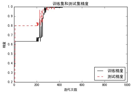
# 展示训练和测试精度
plt.plot(train_accuracy, 'k-', label='训练精度')
plt.plot(test_accuracy, 'r--', label='测试精度')
plt.title('训练集和测试集精度')
plt.xlabel('迭代次数')
plt.ylabel('精度')
plt.legend(loc='lower right')
plt.show()
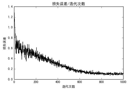
# 损失函数效果
plt.plot(loss_vec, 'k-')
plt.title('损失误差/迭代次数')
plt.xlabel('迭代次数')
plt.ylabel('损失误差')
plt.show()
分类结果展示:
精度效果:
损失误差:
更多干货请关注:
