Softmax & 分类模型

Softmax

与候选采样相对

Softmax function, a wonderful activation function that turns numbers aka logits into probabilities that sum to one. Softmax function outputs a vector that represents the probability distributions of a list of potential outcomes.

一种函数，可提供多类别分类模型中每个可能类别的概率。这些概率的总和正好为 1.0。

Example: softmax 可能会得出某个图像是狗、猫和马的概率分别是 0.9、0.08 和 0.02。（也称为完整 softmax。）在这里插入图片描述

softmax的基本概念

分类问题
一个简单的图像分类问题，输入图像的高和宽均为2像素，色彩为灰度。
图像中的4像素分别记为 $x_1, x_2, x_3, x_4$ 。
假设真实标签为狗、猫或者鸡，这些标签对应的离散值为 $y_1, y_2, y_3$ 。
我们通常使用离散的数值来表示类别，例如 $y_1=1, y_2=2, y_3=3$ 。
权重矢量

$egin{aligned} o_1 &= x_1 w_{11} + x_2 w_{21} + x_3 w_{31} + x_4 w_{41} + b_1 end{aligned}$

$egin{aligned} o_2 &= x_1 w_{12} + x_2 w_{22} + x_3 w_{32} + x_4 w_{42} + b_2 end{aligned}$

$egin{aligned} o_3 &= x_1 w_{13} + x_2 w_{23} + x_3 w_{33} + x_4 w_{43} + b_3 end{aligned}$

神经网络图
下图用神经网络图描绘了上面的计算。softmax回归同线性回归一样，也是一个单层神经网络。由于每个输出 $o_1, o_2, o_3$ 的计算都要依赖于所有的输入 $x_1, x_2, x_3, x_4$ ，softmax回归的输出层也是一个全连接层。

$egin{aligned}softmax回归是一个单层神经网络end{aligned}$

既然分类问题需要得到离散的预测输出，一个简单的办法是将输出值 $o_i$ 当作预测类别是 $i$ 的置信度，并将值最大的输出所对应的类作为预测输出，即输出 $underset{i}{argmax} o_i$ 。例如，如果 $o_1,o_2,o_3$ 分别为 $0.1,10,0.1$ ，由于 $o_2$ 最大，那么预测类别为2，其代表猫。

输出问题
直接使用输出层的输出有两个问题：
1. 一方面，由于输出层的输出值的范围不确定，我们难以直观上判断这些值的意义。例如，刚才举的例子中的输出值10表示“很置信”图像类别为猫，因为该输出值是其他两类的输出值的100倍。但如果 $o_1=o_3=10^3$ ，那么输出值10却又表示图像类别为猫的概率很低。
2. 另一方面，由于真实标签是离散值，这些离散值与不确定范围的输出值之间的误差难以衡量。

softmax运算符（softmax operator）解决了以上两个问题。它通过下式将输出值变换成值为正且和为1的概率分布：

$hat{y}_1, hat{y}_2, hat{y}_3 = ext{softmax}(o_1, o_2, o_3)$

其中

$hat{y}1 = frac{ exp(o_1)}{sum_{i=1}^3 exp(o_i)},quad hat{y}2 = frac{ exp(o_2)}{sum_{i=1}^3 exp(o_i)},quad hat{y}3 = frac{ exp(o_3)}{sum_{i=1}^3 exp(o_i)}.$

容易看出 $hat{y}_1 + hat{y}_2 + hat{y}_3 = 1$ 且 $0 leq hat{y}_1, hat{y}_2, hat{y}_3 leq 1$ ，因此 $hat{y}_1, hat{y}_2, hat{y}_3$ 是一个合法的概率分布。这时候，如果 $hat{y}_2=0.8$ ，不管 $hat{y}_1$ 和 $hat{y}_3$ 的值是多少，我们都知道图像类别为猫的概率是80%。此外，我们注意到

$underset{i}{argmax} o_i = underset{i}{argmax} hat{y}_i$

因此softmax运算不改变预测类别输出。

计算效率
- 单样本矢量计算表达式
  为了提高计算效率，我们可以将单样本分类通过矢量计算来表达。在上面的图像分类问题中，假设softmax回归的权重和偏差参数分别为

$oldsymbol{W} = egin{bmatrix} w_{11} & w_{12} & w_{13} \ w_{21} & w_{22} & w_{23} \ w_{31} & w_{32} & w_{33} \ w_{41} & w_{42} & w_{43} end{bmatrix},quad oldsymbol{b} = egin{bmatrix} b_1 & b_2 & b_3 end{bmatrix},$

设高和宽分别为2个像素的图像样本 $i$ 的特征为

$oldsymbol{x}^{(i)} = egin{bmatrix}x_1^{(i)} & x_2^{(i)} & x_3^{(i)} & x_4^{(i)}end{bmatrix},$

输出层的输出为

$oldsymbol{o}^{(i)} = egin{bmatrix}o_1^{(i)} & o_2^{(i)} & o_3^{(i)}end{bmatrix},$

预测为狗、猫或鸡的概率分布为

$oldsymbol{hat{y}}^{(i)} = egin{bmatrix}hat{y}_1^{(i)} & hat{y}_2^{(i)} & hat{y}_3^{(i)}end{bmatrix}.$

softmax回归对样本 $i$ 分类的矢量计算表达式为

$egin{aligned} oldsymbol{o}^{(i)} &= oldsymbol{x}^{(i)} oldsymbol{W} + oldsymbol{b},\ oldsymbol{hat{y}}^{(i)} &= ext{softmax}(oldsymbol{o}^{(i)}). end{aligned}$

小批量矢量计算表达式
为了进一步提升计算效率，我们通常对小批量数据做矢量计算。广义上讲，给定一个小批量样本，其批量大小为 $n$ ，输入个数（特征数）为 $d$ ，输出个数（类别数）为 $q$ 。设批量特征为 $oldsymbol{X} in mathbb{R}^{n imes d}$ 。假设softmax回归的权重和偏差参数分别为 $oldsymbol{W} in mathbb{R}^{d imes q}$ 和 $oldsymbol{b} in mathbb{R}^{1 imes q}$ 。softmax回归的矢量计算表达式为

$egin{aligned} oldsymbol{O} &= oldsymbol{X} oldsymbol{W} + oldsymbol{b},\ oldsymbol{hat{Y}} &= ext{softmax}(oldsymbol{O}), end{aligned}$

其中的加法运算使用了广播机制， $oldsymbol{O}, oldsymbol{hat{Y}} in mathbb{R}^{n imes q}$ 且这两个矩阵的第 $i$ 行分别为样本 $i$ 的输出 $oldsymbol{o}^{(i)}$ 和概率分布 $oldsymbol{hat{y}}^{(i)}$ 。

两种操作对比

numpy 操作：np.exp(x) / np.sum(np.exp(x), axis=0)
pytorch 操作：torch.exp(x)/torch.sum(torch.exp(x), dim=1).view(-1,1)

引入Fashion-MNIST

为方便介绍 Softmax，为了更加直观的观察到算法之间的差异
引入较为复杂的多分类图像分类数据集

导入：torchvision 包【构建计算机视觉模型】

# import needed package
%matplotlib inline
from IPython import display
import matplotlib.pyplot as plt

import torch
import torchvision
import torchvision.transforms as transforms
import time

import sys
sys.path.append("path to file storge FashionMNIST.zip")
import d2lzh1981 as d2l

# print(torch.__version__)
# print(torchvision.__version__)

# get dataset
mnist_train = torchvision.datasets.FashionMNIST(root='path to file storge FashionMNIST.zip', train=True, download=True, transform=transforms.ToTensor())
mnist_test = torchvision.datasets.FashionMNIST(root='path to file storge FashionMNIST.zip', train=False, download=True, transform=transforms.ToTensor())

def get_fashion_mnist_labels(labels):
    text_labels = ['t-shirt', 'trouser', 'pullover', 'dress', 'coat',
                   'sandal', 'shirt', 'sneaker', 'bag', 'ankle boot']
    return [text_labels[int(i)] for i in labels]
def show_fashion_mnist(images, labels):
    d2l.use_svg_display()
    # 这里的_表示我们忽略（不使用）的变量
    _, figs = plt.subplots(1, len(images), figsize=(12, 12))
    for f, img, lbl in zip(figs, images, labels):
        f.imshow(img.view((28, 28)).numpy())
        f.set_title(lbl)
        f.axes.get_xaxis().set_visible(False)
        f.axes.get_yaxis().set_visible(False)
    plt.show()
X, y = [], []
for i in range(10):
    X.append(mnist_train[i][0]) # 将第i个feature加到X中
    y.append(mnist_train[i][1]) # 将第i个label加到y中
show_fashion_mnist(X, get_fashion_mnist_labels(y))

# read data
batch_size = 256
num_workers = 4
train_iter = torch.utils.data.DataLoader(mnist_train, batch_size=batch_size, shuffle=True, num_workers=num_workers)
test_iter = torch.utils.data.DataLoader(mnist_test, batch_size=batch_size, shuffle=False, num_workers=num_workers)

start = time.time()
for X, y in train_iter:
    continue
print('%.2f sec' % (time.time() - start))

Softmax 手动实现

import package and module

import torch
import torchvision
import numpy as np
import sys
sys.path.append("path to file storge FashionMNIST.zip")
import d2lzh1981 as d2l

print(torch.__version__)
print(torchvision.__version__)

获取数据

batch_size = 256
train_iter, test_iter = d2l.load_data_fashion_mnist(batch_size)

模型参数初始化

# init module param 
num_inputs = 784
print(28*28)
num_outputs = 10

W = torch.tensor(np.random.normal(0, 0.01, (num_inputs, num_outputs)), dtype=torch.float)
b = torch.zeros(num_outputs, dtype=torch.float)
W.requires_grad_(requires_grad=True)
b.requires_grad_(requires_grad=True)

Sofmax 定义

# define softmax function
def softmax(X):
    X_exp = X.exp()
    partition = X_exp.sum(dim=1, keepdim=True)
    # print("X size is ", X_exp.size())
    # print("partition size is ", partition, partition.size())
    return X_exp / partition  # 这里应用了广播机制

softmax 回归模型

# define regression model
def net(X):
    return softmax(torch.mm(X.view((-1, num_inputs)), W) + b)

损失函数

# define loss function
def cross_entropy(y_hat, y):
    return - torch.log(y_hat.gather(1, y.view(-1, 1)))

准确率

def accuracy(y_hat, y):
    return (y_hat.argmax(dim=1) == y).float().mean().item()

训练模型

num_epochs, lr = 5, 0.1

def train_ch3(net, train_iter, test_iter, loss, num_epochs, batch_size,
              params=None, lr=None, optimizer=None):
    for epoch in range(num_epochs):
        train_l_sum, train_acc_sum, n = 0.0, 0.0, 0
        for X, y in train_iter:
            y_hat = net(X)
            l = loss(y_hat, y).sum()
            
            # 梯度清零
            if optimizer is not None:
                optimizer.zero_grad()
            elif params is not None and params[0].grad is not None:
                for param in params:
                    param.grad.data.zero_()
            
            l.backward()
            if optimizer is None:
                d2l.sgd(params, lr, batch_size)
            else:
                optimizer.step() 
            
            
            train_l_sum += l.item()
            train_acc_sum += (y_hat.argmax(dim=1) == y).sum().item()
            n += y.shape[0]
        test_acc = evaluate_accuracy(test_iter, net)
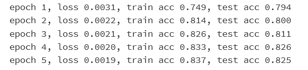
        print('epoch %d, loss %.4f, train acc %.3f, test acc %.3f'
              % (epoch + 1, train_l_sum / n, train_acc_sum / n, test_acc))

train_ch3(net, train_iter, test_iter, cross_entropy, num_epochs, batch_size, [W, b], lr)

模型预测

X, y = iter(test_iter).next()

true_labels = d2l.get_fashion_mnist_labels(y.numpy())
pred_labels = d2l.get_fashion_mnist_labels(net(X).argmax(dim=1).numpy())
titles = [true + '
' + pred for true, pred in zip(true_labels, pred_labels)]

d2l.show_fashion_mnist(X[0:9], titles[0:9])

Pytorch 改进

# import package and module
import torch
from torch import nn
from torch.nn import init
import numpy as np
import sys
sys.path.append("path to file storge FashionMNIST.zip")
import d2lzh1981 as d2l

初始化参数和获取数据

# init param and get data
batch_size = 256
train_iter, test_iter = d2l.load_data_fashion_mnist(batch_size)

定义网络模型

num_inputs = 784
num_outputs = 10

class LinearNet(nn.Module):
    def __init__(self, num_inputs, num_outputs):
        super(LinearNet, self).__init__()
        self.linear = nn.Linear(num_inputs, num_outputs)
    def forward(self, x): # x 的形状: (batch, 1, 28, 28)
        y = self.linear(x.view(x.shape[0], -1))
        return y
    
# net = LinearNet(num_inputs, num_outputs)

class FlattenLayer(nn.Module):
    def __init__(self):
        super(FlattenLayer, self).__init__()
    def forward(self, x): # x 的形状: (batch, *, *, ...)
        return x.view(x.shape[0], -1)

from collections import OrderedDict
net = nn.Sequential(
        # FlattenLayer(),
        # LinearNet(num_inputs, num_outputs) 
        OrderedDict([
           ('flatten', FlattenLayer()),
           ('linear', nn.Linear(num_inputs, num_outputs))]) # 或者写成我们自己定义的 LinearNet(num_inputs, num_outputs) 也可以
        )

初始化模型参数

# init module param
init.normal_(net.linear.weight, mean=0, std=0.01)
init.constant_(net.linear.bias, val=0)

损失函数

loss = nn.CrossEntropyLoss() # 下面是他的函数原型
# class torch.nn.CrossEntropyLoss(weight=None, size_average=None, ignore_index=-100, reduce=None, reduction='mean')

优化函数

optimizer = torch.optim.SGD(net.parameters(), lr=0.1) # 下面是函数原型
# class torch.optim.SGD(params, lr=, momentum=0, dampening=0, weight_decay=0, nesterov=False)

训练

num_epochs = 5
d2l.train_ch3(net, train_iter, test_iter, loss, num_epochs, batch_size, None, None, optimizer)

训练结果分析

在这里插入图片描述

最开始：训练数据集上的准确率低于测试数据集上的准确率

原因

训练集上的准确率是在一个epoch的过程中计算得到的
测试集上的准确率是在一个epoch结束后计算得到的
Result: 后者的模型参数更优

让对手感动，让对手恐惧