Local Search
Systematic algorithms: achieve systematicity by keeping one or more paths in memory and by recording which alternatives have been explored at each point along the path. When a goal is found, the path to that goal also constitutes a solution to the problem.
Local search algorithms: operate using a single current node (rather than multiple paths) and generally move only to neighbors of that node. Typically, the path followed by the search are not retained.
Optimization problems: Local search algorithms are useful for solving pure optimization problems, in which the aim is to find the best state according to an objective function.
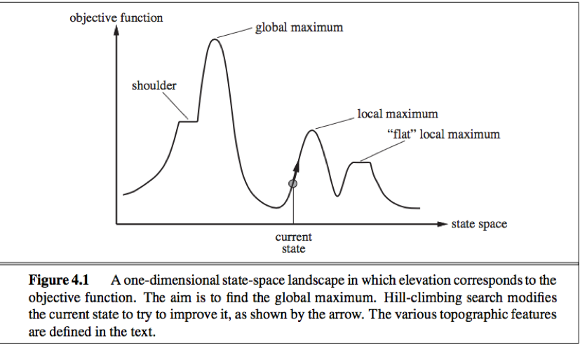
State-space landscape: Local search algorithms explore a landscape that has both “location”(defined by the state) and “elevation”(defined by the value of the heuristic cost function or objective function).
If elevation corresponds to cost, the aim is to find the lowest valley—a global minimum;
If elevation corresponds to an objective function, the aim is to find the highest peak—a global maximum.(can convert from one to the other by inserting a minus sign).
A complete local search algorithm always finds a goal if one exists, an optimal algorithm always finds a global minimum/maximum.
1. Hill-climbing search:
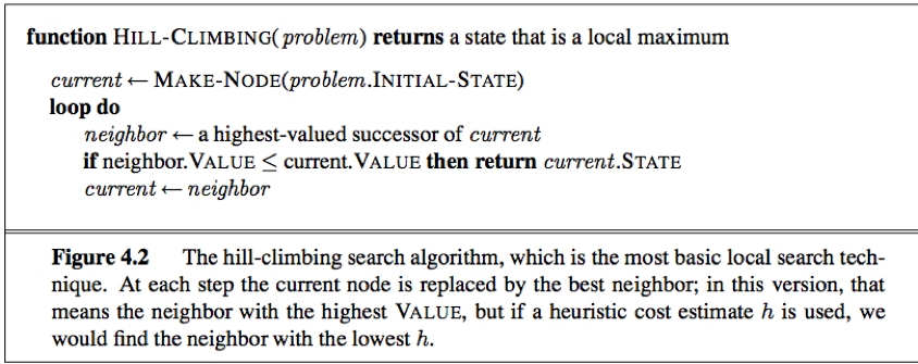
Hill-climbing search algorithm(steepest-ascent version): A loop continually moves in the direction of increasing value(uphill), terminates when it reaches a “peak” where no neighbor has a higher value.
The algorithm does not maintain a search tree, so the data structure for the current node only record the state and the value of the objective function.
Hill climbing often get stuck for the following reasons:
1. Local maxima: Hill-climbing algorithms that reach the vicinity of a local maximum will be drawn upward toward a local maximum but then be stuck.
2. Ridges: Ridges result in a sequence of local maxima that are not directly connected to each other.
3. Plateaux: A flat area of the state-space landscape, can be flat local maximum(no uphill exit exists) or shoulder(progress is possible).
When the algorithm halts at a plateau, we should take care to allow sideways moves (in the hope that the plateau is a shoulder), and put a limit on the number of consecutive sideways move allowed to avoid infinite loop.
Local search methods such as hill climbing operate on complete-state formulations, keeping only a small number of nodes in memory.
Variants of hill climbing:
1. Stochastic hill climbing: chooses at random from among the uphill moves, the probability of selection vary with the steepness of the uphill move.
2. First-choice hill climbing: implements stochastic hill climbing by generating successors randomly until one is generated that is better than the current state.
3. Random-restart hill climbing: conducts a series of hill-climbing searches from randomly generated initial states, until a goal is found.(complete)
2. Simulated annealing
Simulated annealing: switch from hill climbing to gradient descent(i.e. minimizing cost), start by shaking hard (hard enough bounce out of local minima), and then gradually reduce the intensity of the shaking(not hard enough to dislodge from the global minimum).
The algorithm picks a random move.
If the move improves the situation, it is always accepted;
Otherwise accepts the move with probability <1, the probability decreases exponentially with △E↑ and T↓.
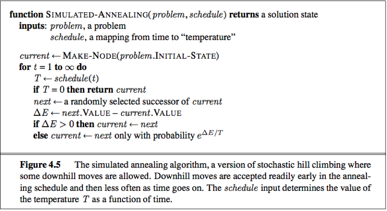
Simulated annealing is a stochastic algorithm, it returns optimal solutions when given an appropriate cooling schedule.
3. Local beam search
Local beam search: The local beam search algorithm keeps track of k states rather than just one.
It begins with k randomly generated states, at each step, all successors of all states are generated. If any one is a goal, the algorithm halts; Otherwise it selects the k best successors from the complete list and repeat.
Different from random-restart algorithm:
In a random-restart search, each search process runs independently of the others;
In a local beam search, useful information is passed among the parallel search threads, quickly abandons unfruitful searches and moves its resources to whre the most progress is being made.
Stochastic beam search: a variant analogous to stochastic hill climbing, alleviate the problem of a lack of diversity among the k states. Stochastic beam search chooses k successors at random with probability of choosing a given successor being an increasing function of its value.
4. Genetic algorithms
Genetic algorithm: A genetic algorithm (GA) is a variant of stochastic beam search. Successor states are generated by combining two parent states.
A genetic algorithm is a stochastic hill-climbing search in which a large population of states is maintained. New states are generated by mutation and by crossover, which combines pairs of states from the population.
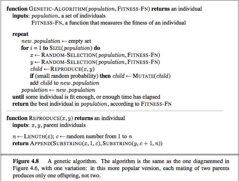
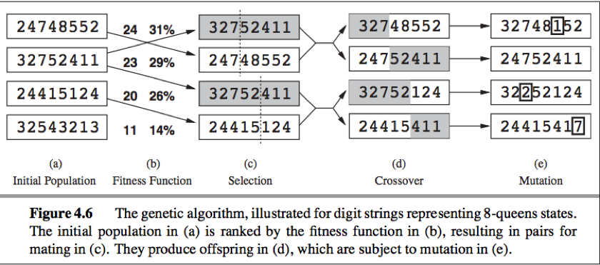
(a) GA begin with a set of k randomly generated states(population), each state(individual) is represented as a string over a finite alphabet.
(b) Each state is rated by the objective function (the fitness function). A fitness function should return higher values for better states.
(c) pairs are selected at random for reproduction in accordance with the probabilities. (have many variants, exp: culling instead of random). For each pair a crossover point is chosen randomly from the position in the string.
(d) cross over the parent strings at the crossover point to create offspring.
Crossover frequently takes large steps in the state space early in the search process and smaller steps later on.
(e) Each location is subject to random mutation with a small independent probability.
Schema: A substring in which some of the positions can be left unspecified(exp:246*****). String that match the schema are called instances of the schema.
If the average fitness of the instances of a schema is above the mean, then the number of instances of the schema within the population will grow over time.
Local search in continuous spaces
The states are defined by n variables (defined by an n-dimensional vector of variables x.)
Gradient of the objective function ▽f
Local expression for the gradient 
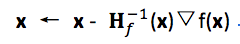
Can perform steepest-ascent hill climbing by updating the current state according to the formula x ← x + α▽f(x) , αis the step size (a small constant).
If the objection function f is not available in a differentiable form, use empirical gradient search.
Line search: tries to overcome the dilemma of adjusting α by extending the current gradient direction—repeatedly doubling αuntil f starts to decrease again. The point at which this occurs becomes the new current state.
In cases that the objective function is not differentiable: we calculate an empirical gradient by evaluating the response to small increments and decrements in each coordinate. Empirical gradient search is the same as steepest-ascent hill climbing in a discretized version of the state space.
Newton-Raphson method:
Hf(x) is the Hessian matrix of second derivatives, Hij = 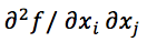
Constrained optimization: An optimization problem is constrained if solutions must satisfy some hard constraints on the values of the variables. (e.g. : linear programming problems)
Many local search methods apply also to problems in continuous spaces. Linear programming and convex optimization problems obey certain restrictions on the shape of the state space and the nature of the objective function, and admit polynomial-time algorithms that are oftenly extremely efficient in practice.
Searching with nondeterministic actions
When the environment is either partially observable or nondeterministic (or both), the future percepts cannot be determined in advance, and the agent’s future actions will depend on those future percepts.
Nondeterministic problems:
Transition model is defined by RESULTS function that returns a set of possible outcome states;
Solution is not a sequence but a contingency plan (strategy),
e.g.
[Suck, if State = 5 then [Right, Suck] else []];
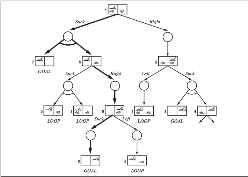
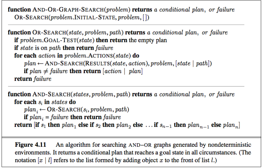
In nondeterministic environments, agents can apply AND-OR search to generate contingent plans that reach the goal regardless of which outcomes occur during execution.
AND-OR search trees
OR nodes: In a deterministic environment, the only branching is introduced by the agent’s own choices in each state, we call these nodes OR nodes.
AND nodes: In a nondeterministic environment, branching is also introduced by the environment’s choice of outcome for each action, we call these nodes AND nodes.
AND-OR tree: OR nodes and AND nodes alternate. States nodes are OR nodes where some action must be chosen. At the AND nodes (shown as circles), every outcome must be handled.
A solution (shown in bold lines) for an AND-OR search problem is a subtree that
1) has a goal node at every leaf;
2) specifies one action at each of its OR nodes;
3) includes every outcome branch at each of its AND nodes.
A recursive, depth-first algorithm for AND-OR graph search
Cyclic solution
Cyclic solution: keep trying until it works. We can express this solution by adding a label to denote some portion of the plan and using the label later instead of repeating the plan itself. E.g.: [Suck, L1: Right, if State = 5 then L1 else Suck]. (or “while State = 5 do Right”).
Searching with partial observatioins
Belief state: The agent's current belief about the possible physical states it might be in, given the sequence of actions and percepts up to that point.
Standard search algorithms can be applied directly to belief-state space to solve sensorless problems, and belief-state AND-OR search can solve general partially observable problems. Incremental algorithms that construct solutions state-by-state within a belief state are often more efficient.
1. Searching with no observation
When the agent's percepts provide no information at all, we have a sensorless problem.
To solve sensorless problems, we search in the space of belief states rather than physical states. In belief-state space, the problem is fully observable, the solution is always a sequence of actions.
Belief-state problem can be defined by: (The underlying physical problem P is defined by ACTIONSP, RESULTP, GOAL-TESTP and STEP-COSTP)
·Belief states: Contains every possible set of physical states. If P has N states, the sensorless problem has up to 2^N states (although many may be unreachable from the initial state).
·Initial states: Typically the set of all states in P.
·Actions:
a. If illegal actions have no effect on the environment, take the union of all the actions in any of the physical states in the current belief b:
ACTIONS(b) =![]()
b. If illegal actions are extremely dangerous, take the intersection.
·Transition model:
a. For deterministic actions,
b' = RESULT(b,a) = {s' : s' = RESULTP(s,a) and s∈b}. (b' is never larger than b).
b. For nondeterministic actions,
b' = RESULT(b,a) = {s' : s' = RESULTP(s,a) and s∈b} = (b' may be larger than b)
The process of generating the new belief state after the action is called the prediction step.
·Goal test: A belief state satisfies the goal only if all the physical states in it satisfy GOAL-TESTP.
·Path cost
If an action sequence is a solution for a belief state b, it is also a solution for any subset of b. Hence, we can discard a path reaching the superset if the subset has already been generated. Conversely, if the superset has already been generated and found to be solvable, then any subset is guaranteed to be solvable.
Main difficulty: The size of each belief state.
Solution:
a. Represent the belief state by some more compact description;
b. Avoid the standard search algorithm, develop incremental belief state search algorithms instead.
Incremental belief-state search: Find one solution that works for all the states, typically able to detect failure quickly.
2. Searching with observations
When observations are partial, The ACTIONS, STEP-COST, and GOAL-TEST are constructed form the underlying physical problem just as for sensorless problems.
·Transition model: We can think of transitions from one belief state to the next for a particular action as occurring in 3 stages.
The prediction stage is the same as for sensorless problem, given the action a in belief state b, the predicted belief state is ![]()
The observation prediction stage determines the set of percepts o that could be observed in the predicted belief state:
![]()
The update stage determines, for each possible percept, the belief state that would result from the percept. The new belief state bo is the set of states in ![]() that could have produced the percept:
that could have produced the percept:
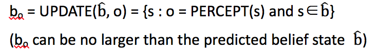
In conclusion:
RESULTS(b,a) = { bo : bo = UPDATE(PREDICT(b,a),o) and o∈POSSIBLE-PERCEPTS(PREDICT(b,a))}
Search algorithm return a conditional plan that test the belief state rather than the actual state.
Agent for partially observable environments is similar to the simple problem-solving agent (formulates a problem, calls a search algorithm, executes the solution).
Main difference:
1) The solution will be a conditional plan rather than a sequence.
2) The agent will need to maintain its belief state as it performs actions and receives percepts.
Given an initial state b, an action a, and a percept o, the new belief state is
b’ = UPDATE(PREDICT(b, a), o). //recursive state estimator
Sate estimation: a.k.a. monitoring or filtering, a core function of intelligent system in partially observable environments—maintaining one’s belief state.
Online search Agents
Online search is a necessary idea for unknown environments. Online search agent interleaves computation and action: first it takes an action, then it observes the environment and computes the next action.
1. Online search problem
Assume a deterministic and fully observable environment, the agent only knows:
·ACTION(s): returns a list of actions allowed in state s;
·c(s, a, s’): The step-cost function, cannot be used until the agent knows that s’ is the outcome;
·GOAL-TEST(s).
·The agent cannot determine RESULT(s, a) except by actually being in s and doing a.
·The agent might have access to an admissible heuristic function h(s) that estimates the distance from the current state to a goal state.
Competitive ratio: The cost (the total path cost of the path that the agent actually travels) / the actual shortest path (the path cost of the path the agent would follow if it knew the search space in advance). The competitive ratio is expected to be as small as possible.
In some case the best achievable competitive ratio is infinite, e.g. some actions are irreversible and might reach a dead-end state. No algorithm can avoid dead ends in all state spaces.
Safely explorable: some goal state is reachable from every reachable state. E.g. state spaces with reversible actions such as mazes and 8-puzzles.
No bounded competitive ratio can be guaranteed even in safely explorable environments if there are paths of unbounded cost.
2. Online search agents

ONLINE-DFS-AGENT works only in state spaces where the actions are reversible.
RESULT: a table the agent stores its map, RESULT[s, a] records the state resulting from executing action a in state s.
Whenever an action from the current sate has not been explored, the agent tries that action.
When the agent has tried all the actions in a state, the agent in an online search backtracks physically (in a depth-first search, means going back to the state from which the agent most recently entered the current sate).
3. Online local search
Exploration problems arise when the agent has no idea about the satate and actions of its environment. For safely explorable environments, online search agents can build a map and find a goal if one exists. Updating heuristic estimates from experience provides an effective method to escape from local minima.
Random walk: Because online hill-climbing search cannot use restart(because the agent cannot transport itself to a new state), can use random walk instead. A random walk simply selects at random one of the available actions from the current state, preference can be given to actions that have not yet been tried.
Basic idea of online agent: Random walk will eventually find a goal or complete its exploration if the space is finite, but can be very slow. A more effective approach is to store a “current best estimate” H(s) of the cost to reach the goal from each state that has been visited. H(s) starts out being the heuristic estimate h(s) and is updated as the agent gains experience in the state space.
If the agent is stuck in a flat local minimum, the agent will follow what seems to be the best path to the goal given the current cost estimates for its neighbors. The estimate cost to reach the goal through a neighbor s’ is the cost to get to s’ plus the estimated cost to get to a goal from there, that is, c(s, a, s') + H(s').
LRTA*: learning real-time A*. It builds a map of the environment in the result table, update the cost estimate for the state it has just left and then chooses the “apparently best” move according to its current cost estimates.
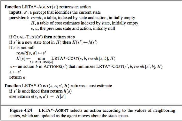
Actions that have not yet been tried in a state s are always assumed to lead immediately to the goal with the least possible cost (a.k.a.h(s)), this optimism under uncertainty encourages the agent to explore new, possible promising paths.