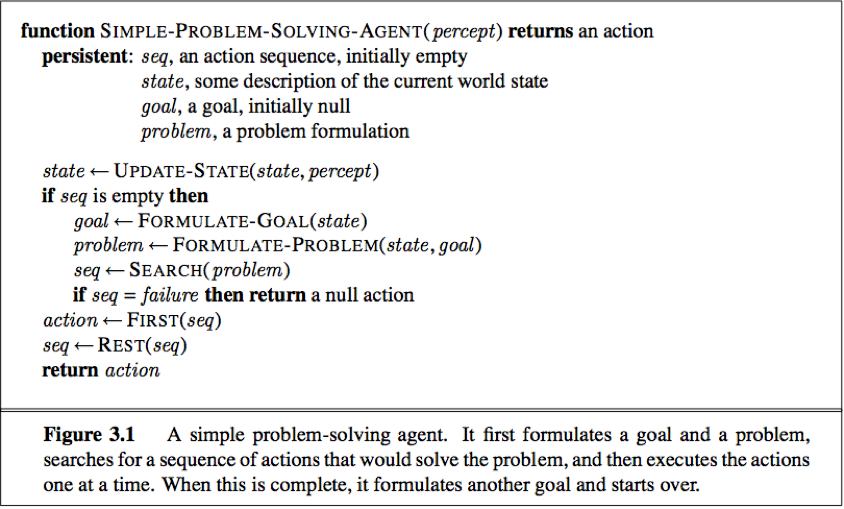
Problem-solving agent: one kind of goal-based agent using atomic representation.
Problem formulation: the process of deciding what actions and states to consider, given a goal.
Search: the process of looking for a sequence of actions that reaches the goal.
A problem can be defined formally by 5 components(The input to a problem-solving algorithm):
1. The initial state(the state that the agent starts in)
2. A description of the possible action available to the agent.
ACTION(s) returns the set of actions that can be executed in state s, exp:
ACTION(In(Arad)) = {Go(Sibiu), Go(Timisoara), Go(Zerind)}.
3. The transition model(A description of what each action does).
Function RESULT(s, a) returns the state that results from doing action a in state s. exp:
RESULT(In(Arad), Go(Zerind)) = In(Zerind).
4. The goal test(determines whether a given state is a goal state).
5. A past cost function (assigns a numeric cost to each path).
A solution to a problem is an action sequence that leads from the initial state to a goal state, an optimal solution has the lowest path cost among all solutions.
TREE-SEARCH
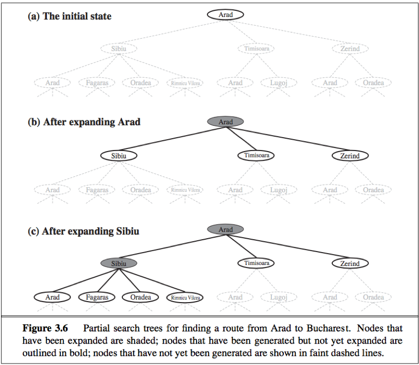
TREE-SEARCH: The possible action sequences starting at the initial state form a search tree with the initial state at the root, the branches are actions and the nodes correspond to states in the state space of the problem.
Follow up one option now and put the other aside for later in case the first choice does not lead to a solution--choose a node first, check to see whether it is a goal state(it is not) and then expand the current state(applying each legal action thereby generate a new set of states, add branches from the parent node leading to new child nodes), then choose which of these possibilities to consider further.
A leaf node is a node with no children in the tree, the set of all leaf nodes available for expansion at any given point is called the frontier(open list).
The process of expanding nodes on the frontier continues until either a solution is found or there are no more states to expand.
GRAPH-SEARCH:
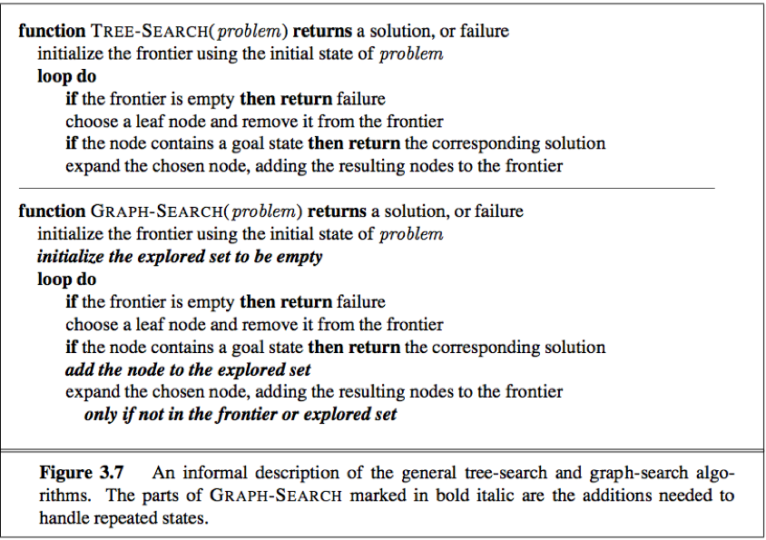
GRAPH-SEARCH: to avoid exploring redundant paths, we augment the TREE-SEARCH algorithm with a data structure called the explored set(a.k.a. closed list), which remembers every expanded node. Newly generated nodes that match previously generated nodes—ones in the explored set or the frontier—can be discarded instead of being added to the frontier.
(The explored set can be implemented with a hash table to allow efficient checking for repeated states).
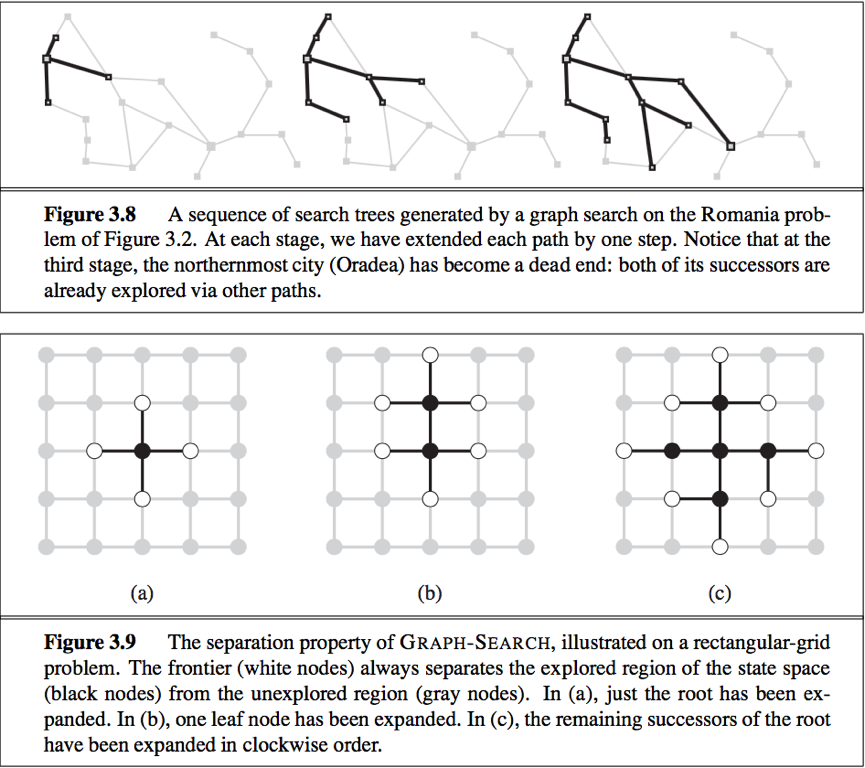
The search tree constructed by the GRAPH-SEARCH algorithm contains at most one copy of each state, so we can think of it as growing a tree directly on the state-space graph.
The GRAPH-SEARCH algorithm has a property: the frontier separates the state-space graph into the explored region and the unexplored region, so that every path from the initial state to an unexplored state has to pass through a state in the frontier.
Infrastructure for search algorithms
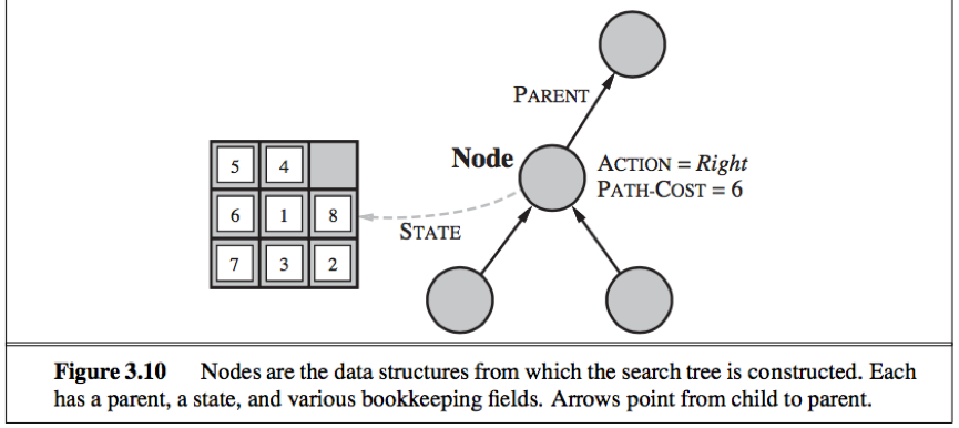
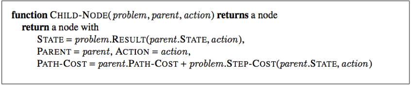
For each node n of the tree, we have a structure that contains 4 components:
1. n.STATE: the state in the state space to which the node corresponds;
2. n.PARENT: the node in the search tree that generated this node;
3. n.ACTION: the action that was applied to the parent to generate the node;
4. n.PATH-COST: denoted by g(n), the cost of the path from the initial state to the node, as indicated by the parent pointers.
A queue is the appropriate data structure for the frontier to be stored in that the search algorithm can easily choose the next node to expand according to its preferred strategy. Operations on a queue includes:
1. EMPTY?(queue): returns true only if there are no more elements in the queue.
2. POP(queue): removes the first element of the queue and returns it.
3. INSERT(element, queue): inserts an element and returns the resulting queue.
Three common variants of queue:
1. FIFO queue: first-in, first-out, pops the oldest element of the queue.
2. LIFO queue(stack): last-in, first-out, pops the newest element of the queue.
3. priority queue: pops the element of the queue with the highest priority according to some ordering function.
Mesuring problem-solving performance
We can evaluate an algorithm’s performance in 4 ways:
1. Completeness: Is the algorithm guaranteed to find a solution when there is one?
2. Optimality: Does the strategy find the optimal solution?
3. Time complexity: How long does it take to find a solution?
4. Space complexity: How much memory is needed to perform the search?
Complexity is expressed in terms of 3 quantities:
1. b, the branching factor or maximum number of successors of any node;
2. d, the depth of the shallowest goal node(i.e., the number of steps along the path from the root);
3. m, the maximum length of any path in the state space.
Uniform search strategies
Uniformed search(blind search): the strategies have no additional information about states beyond that provided in the problem definition, all they can do is generate successors and distinguish a goal state from a non-goal state.
Breadth-first search: the root node is expanded first, then all the successors of the root node are expanded next, then their successors, and so on. All nodes are expanded at a given depth in the search tree before any nodes at the next level are expanded.
In breadth-first search, the shallowest unexpanded node is chosen for expansion. This is achieved by using a FIFO queue for the frontier, thus new nodes(deeper) go to the back of the queue, old nodes(shallower) get expanded first.
The goal test is applied to each node when is generated rather than when it is selected for expansion.(different from the general graph-search algorithm).
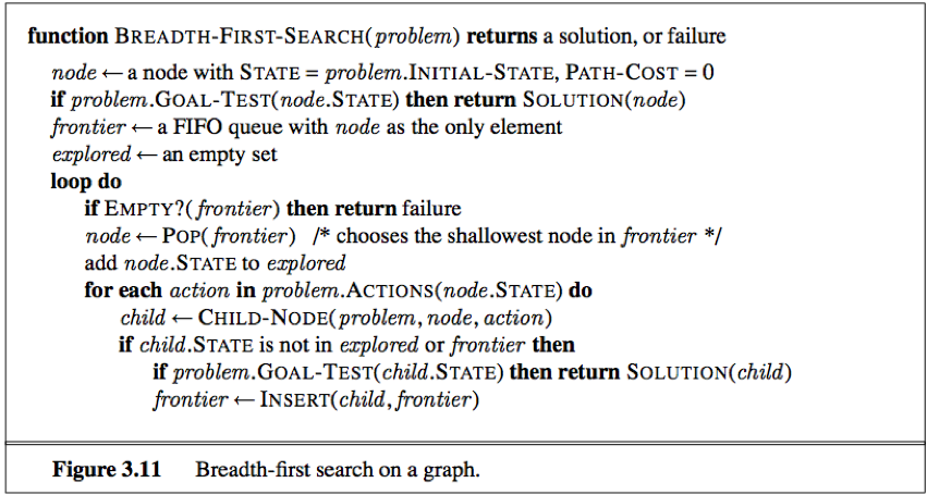
Breadth-first search rate is:
complete if the shallowest goal node is at some finite depth d.
optimal if the past cost is a nondecreasing function of the depth of the node.
Time complexity: O(bd), if every state has b successors and the solution is at depth d.
Space complexity: O(bd).
Uniform-cost search: expands the node n with the lowest past cost g(n), this is done by storing the frontier as priority queue ordered by g.
The goal test is applied to a node when it is selected for expansion rather than when it is first generated,(same as the generic graph-search algorithm), because the first goal node generated may be on a suboptimal path.
A test is added in case a better path is found to a node currently on the frontier.
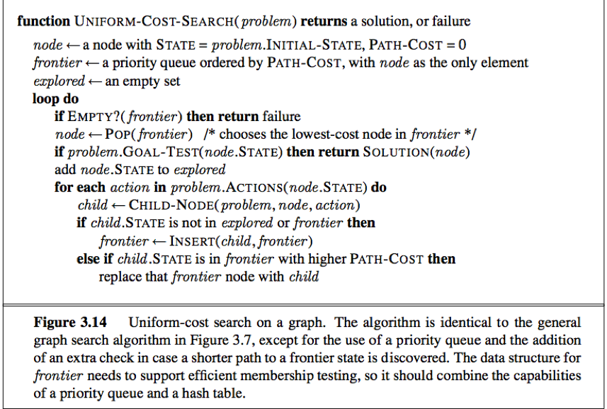
Uniform-cost search is:
Optimal in general.
Complete if the cost of every step exceeds some small positive constant ∊.
Time and space complexity:O,
C* be the cost of the optimal solution, every action costs at least ∊.
Depth-first search: always expands the deepest node in the current frontier of the search tree. The search proceeds immediately to the deepest level of the search tree, where the nodes have no successors. As those nodes are expanded, they are dropped from the frontier, so then the search “backs up” to the next deepest node that still has unexplored successors.
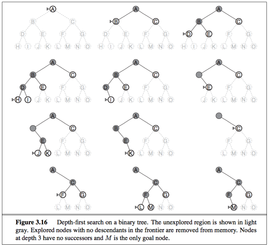
Depth-first-search uses a LIFO queue, that the most recently generated node is chosen for expansion(this must be the deepest unexpanded node).
The properties of depth-first search depend on whether the graph-search or tree-search version is used:
In finite state spaces, the graph-search version is complete, the tree-search version is not complete;
In infinite state spaces, both versions fail if an infinite non-goal path is encountered;
Both versions are nonoptimal;
Time complexity: bounded by the size of the state space(graph search), O(bm),m is the maximum depth of any node(tree search).
Space complexity: O(bm), for a state space with branching factor b and maximum depth m.
[advantage in space complexity: For a graph search, there is no advantage, but a depth-first tree search needs to store only a single path from the root to a leaf node, along with the remaining unexpanded sibling nodes for each node on the path. Once a node has been expanded, it can be removed from memory as soon as all its descendants have been fully explored.]
Dpeth-limited search: supply depth-first search with a predetermined depth limit l(nodes at depth are treated as if they have no successors), thus solves the infinite-path problem of depth-first search.
Depth-limited search can terminate with 2 kinds of failure: the standard failure value indicates no solution; the cutoff value indicates no solution within the depth limit.
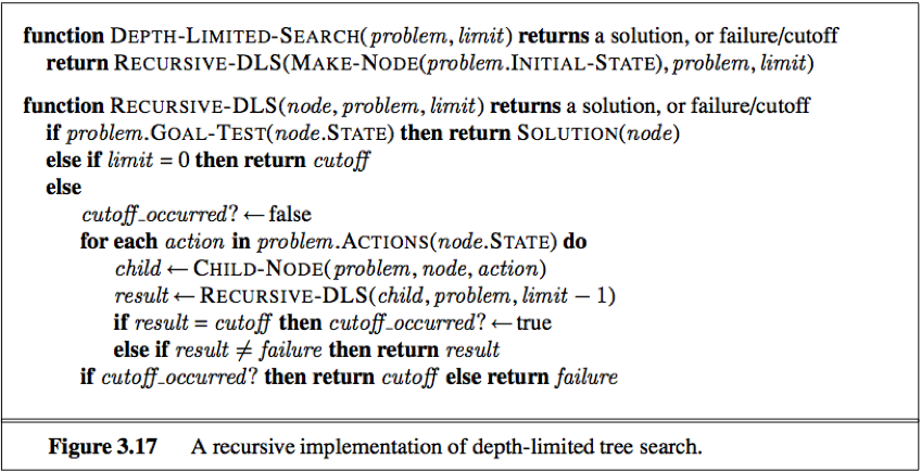
Incomplete if choose l<d, the shallowest goal is beyond the depth limit.
Nonoptimal if l>d
Time complexity: O(bl)
Space complexity: O(bl)
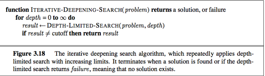
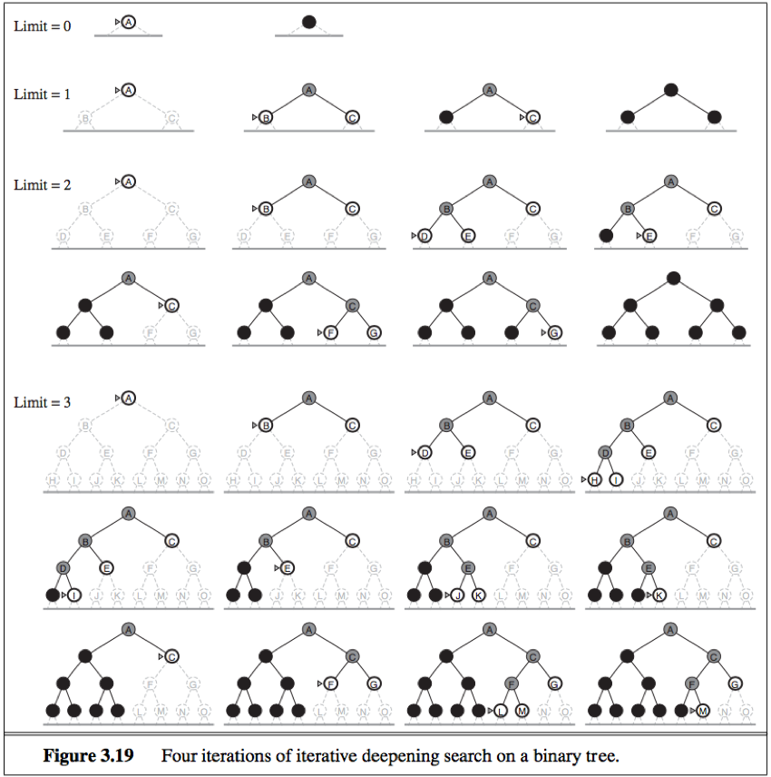
Iterative deepening depth-first search(Iterative deepening search): often used in combination with depth-first tree search to find the best depth limit. It gradually increase the limit(0, 1, 2 …) until a goal is found(when the depth limit reaches d, the depth of the shallowest goal node).
Memory requirements: O(bd)
Complete when the branching factor is finite.
Optimal when the path cost is a nondecreasing function of the depth of the node.
Time complexity: O(bd)
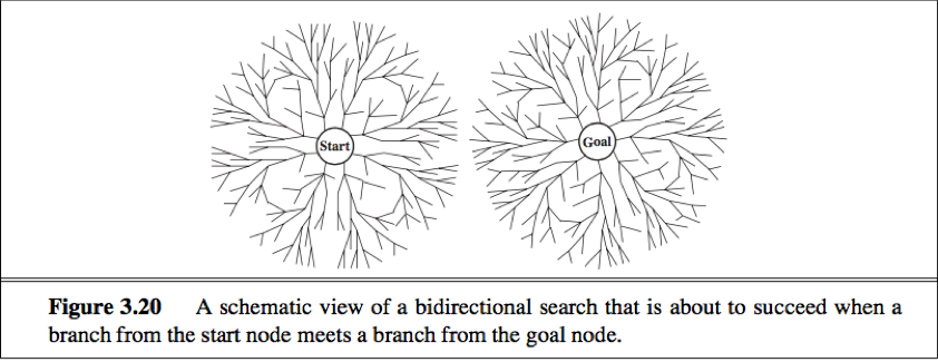
Bidirectional search: run two simultaneous searches—one forward from the initial state and the other backward from the goal—hoping the two searches meet in the middle.
Bidirectional search is implemented by replacing the goal test with a check to see whether the frontiers of the two searches intersect, if they do, a solution has been found.
The first solution found may not be optimal.
Time complexity: O(bd/2) (using breadth-first search in both directions)
Space complexity: O(bd/2) (using breadth-first search in both directions)
Comparing uninformed search strategies fpr tree-search version
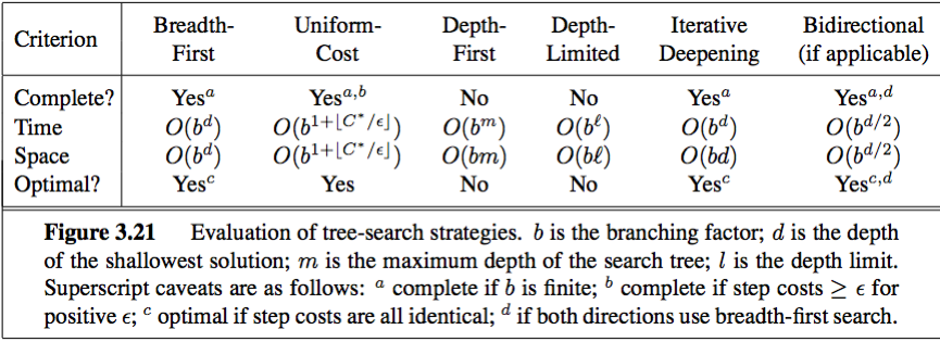
For graph searches, the main differences are that depth-first search is complete for finite state spaces and that the space and time complexities are bounded by the size of the state space.
Informed (heuristic) search strategies
Informed (heuristic) search strategy: uses problem-specific knowledge beyond the definition of the problem itself.
Best first search: an instance of the general TREE-SEARCH or GRAPH-SEARCH algorithm in which a node is selected for expansion based on an evaluation function, f(n).
The evaluation function is constructed as a cost estimate, so the node with the lowest evaluation is expanded first.
The implementation of best-first graph search is identical to that for uniform-cost search, except for the use of f instead of g to order the priority queue.
Most best-first algorithms include as a component of f a heuristic function h(n):
h(n) = estimated cost of the cheapest path from the state at node n to a goal state
unlike g(n), h(n) depends only on the state at that node.
For now, we consider h(n) to be arbitrary, nonnegative, problem-specific function, with one constraint: if n is a goal node, then h(n) = 0.
Greedy best-first search: tries to expand the node that is closest to the goal, on the grounds that this is likely to lead to a solution quickly. f(n) = h(n). At each step it tries to get as close to the goal as it can.
Greedy best-search for tree version is:
incomplete(even in a finite state space)
Worst time and space complexity: O(bm), m is the maximum depth of the search space.
A* search: minimize f(n) = g(n) + h(n)
g(n): the past cost from the start node to reach node n
h(n): the estimated cost of the cheapest path from node n to the goal.
Identical to UNIFORM-COST-SEARCH except that A* uses g+h instead of g.
Conditions for optimality: The tree-search version of A* is optimal if h(n) is admissible, while the graph-search version is optimal if h(n) is consistent.
1.Adimissibility: h(n) be an admissible heuristic.
An admissible heuristic is one that never overestimates the cost to reach the goal. (exp: straight-line distance).
2. Consistency(monotonicity):
A heuristic h(n) is consistent if, for every node n and every successor n’ of n generated by any action a, the estimated cost of reaching the goal from n is no greater than the step cost of getting to n’ plus the estimated cost of reaching the goal from n’:
h(n) <= c(n, a, n’) + h(n’)
Every consistent heuristic is also admissible.
The sequence of nodes expanded by A* using GRAPH-SEARCH is in nondecreasing order of f(n), hence the first goal node selected for expansion must be an optimal solution.
Completeness requires that there be only finitely many nodes with cost less than or equal to C*(the cost of the optimal solution path), a condition that is true if all step costs exceed some finite ∊ and if b is finite.
A* expands no node with f(n)>C*, the algorithm can safely prune(eliminate possibilities from consideration without having to exam them) certain subtree while still guaranteeing optimality.
A* is optimally efficient for any given consistent heuristic—no other algorithm is guaranteed to expand fewer nodes than A*.
Drawback: complexity(mainly in space), A* is not practical for many large-scale problems.
Memory-bounded heuristic search:
1. IDA* algorithm: Iterative-deepening A* algorithm is simplest way to reduce memory requirements for A*, adapt the idea of iterative deepening to the heuristic search context.
Different from standard iterative deepening: At each iteration, the cutoff value is the smallest f-cost of any node that exceeded the cutoff on the previous iteration.
2. RBFS algorithm: Recursive best-first search is a simple recursive algorithm that attempts to mimic the operation of standard best-first search but using only linear space.
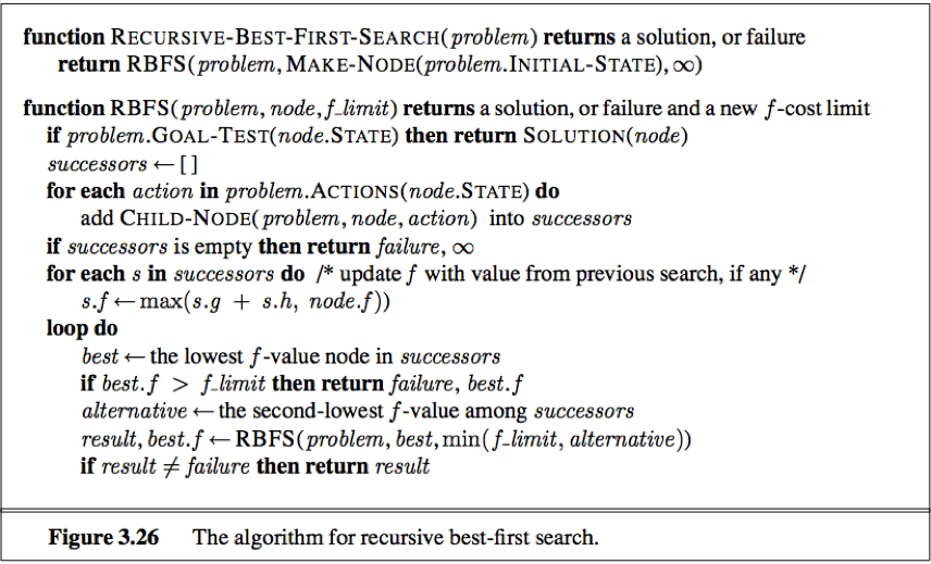
It uses the f_limit variable to keep track of the f-value of the best alternative path available from any ancestor of the current node. If the current node exceeds this limit, the recursion unwinds back to the alternative path and replaces the f-value of each node along the path with a backed-up value(the best f-value of its children). Thus RBFS remembers the f-value of the best leaf in the forgotten subtree to decide whether it’s worth reexpanding the subtree at some later time.
Optimal if the heuristic function h(n) is admissible.
Space complexity: linear in the depth of the deepest optimal solution
Time complexity: depends on the accuracy of h(n) and how often the best path changes as nodes are expanded.
Drawbacks:1. Make use of too little memory(only linear space even if more memory were available) 2. May end up reexpanding the same states many times over. 3. Potentially exponential increase in complexity associated with redundant paths in graphs.
3. SMA*(simplified MA*): proceeds like A*, expanding the best leaf until memory is full(then it cannot add a new node to the search tree without dropping an old one). Always drop the worst leaf node( the one with the highest f-value), then backs up the value of the forgotten node to its parents(like RBFS). Thus SMA* regenerates the subtree only when all other paths have been shown to look worse than the path it has forgotten.
SMA expands the newest best leaf and deletes the oldest worst leaf. When there is only one leaf but the leaf is not a goal node, the node can be discarded.
SMA* is complete if there is any reachable solution(if d, the depth of the shallowest goal node<=the memory size).
Optimal if any optimal solution is reachable.
Metalevel state space: Each state in a metalevel state space captures the internal state of a program that is searching in an object-level state space.(Exp: the internal state of A* algorithm consists of the current search tree.) Each action in the metalevel state space is a computation step that alters the internal state.
A metalevel learning algorithm can learn from experiences to avoid exploring unpromising subtrees.
The effect of heuristic accuracy on performance
Effective branching factor b*: One way to characterize the quality of a heuristic. If the total number of nodes generated by A* for a particular problem is N and the solution depth is d, then b* is the branching factor that a uniform tree of depth d would have to have in order to contain N+1 nodes.
N + 1 = 1 + b* + (b*)2 + … + (b*)d.
A well-designed heuristic would have a value of b* close to 1.
If for any node n, h2(n)>=h1(n), we say h2 donimnates h1—A* using h2 will never expand more nodes than A* using h1.(except some nodes with f(n)=C*).
Generating admissible heuristics from relaxed problems
Relaxed problem: A problem with fewer restriction on the action.
The cost of an optimal solution to a relaxed problem is an admissible and consistent heuristic for the original problem.
If a collection of admissible heuristic h1 … hm is available for a problem and none of them dominates any of the others, we can choose the most accurate function on the node in this question: h(n)=max {h1(n), … , hm(n)}, h is admissible, consistent and dominates all of its component heuristics.
Pattern databases: to store exact solution costs for every possible subproblem instance, then compute an admissible heuristic hDB for each complete state encountered during a search simply by looking up the corresponding subproblem configuration in the database. The database itself is constructed by searching back from the goal and recording the cost of each new pattern encountered; The expense of this search is amortized over many subsequent problem instances.