注:该文是上了开智学堂数据科学基础班的课后做的笔记,主讲人是肖凯老师。
数据操作
数据整理和 Pandas
数据整理是数据分析之前必要的工作。
数据整理包括:
-
数据的基本清洁。如气温数据后面带摄氏度标志 ℃,这时可能需要把符号 ℃ 去掉。
-
数据的拆分合并。有些数据只需要一部分子集,或者需要合并两个不同的数据源。
-
数据转换。如把华氏度转成摄氏度,或者把连续值转成离散值。
-
数据构造。有时需要重新构造新的数据。如体重除以身高,可得到人的身体健康指数。
Pandas 是基于 Numpy 构建的,使以 Numpy 为中心的应用变得更加简单。它的两个主要数据结构是:Series 和 DataFrame。
Series 是一种类似于一维数组的对象,它由一组数据和一组索引组成。
%matplotlib inline
import matplotlib.pyplot as plt;
import numpy as np
import pandas as pd
obj = pd.Series([4, 7, 5, 3])  # 仅由一个数组即可产生最简单的 Series
obj
0    4
1    7
2    5
3    3
dtype: int64
没有为数组指定索引时,就会自动创建一个 0 到 N-1 的整数型索引。可以通过 Series 的 values 和 index 属性获取其数组和索引对象。
obj.values
array([4, 7, 5, 3])
obj.index
RangeIndex(start=0, stop=4, step=1)
除了方便的索引功能,还有汇总和计算描述统计。
obj.median(), obj.mean(), obj.std(), obj.min(), obj.max()
(4.5, 4.75, 1.707825127659933, 3, 7)
obj.describe()
count    4.000000
mean     4.750000
std      1.707825
min      3.000000
25%      3.750000
50%      4.500000
75%      5.500000
max      7.000000
dtype: float64
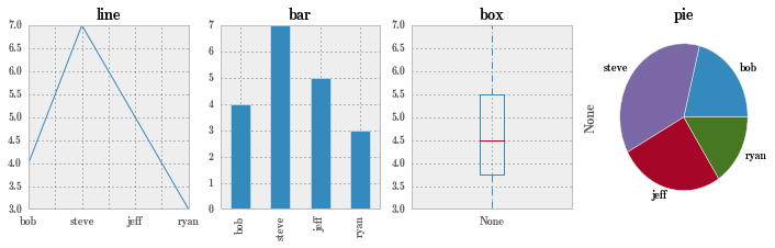
Series 还可绘图。
pd.set_option('display.mpl_style', 'default')
fig, axes = plt.subplots(1, 4, figsize=(12, 3))

obj.plot(ax=axes[0], kind='line', title='line');
obj.plot(ax=axes[1], kind='bar', title='bar');
obj.plot(ax=axes[2], kind='box', title='box');
obj.plot(ax=axes[3], kind='pie', title='pie');
- 如何理解 Series 对象,它和 numpy.array 有何异同?
Series 跟 numpy.array 不一样的地方是,它有 index 属性,即行索引,也可叫行编号。
Series 本质上是一个 Numpy 的数组,因此 Numpy 的数组处理函数可直接用于 Series。但 Series 除了使用位置作为下标提取元素外,还可以使用 index 存取元素。
obj.index = ['bob', 'steve', 'jeff', 'ryan']
print obj[2], obj['jeff']
5 5
和 numpy.array 一样,Series也可以使用一个位置列表或者位置数组进行存取;同时还可以使用 index 列表和 index 数组。
print obj[[0,2,3]]
print obj[['bob','jeff','ryan']]
bob     4
jeff    5
ryan    3
dtype: int64
bob     4
jeff    5
ryan    3
dtype: int64
Series 也支持一些字典的方法,例如 Series.iteritems()。
print list(obj.iteritems())
[('bob', 4), ('steve', 7), ('jeff', 5), ('ryan', 3)]
Series 还集成了绘图功能。
- 如何创建 Series,你能想到几种方法?
obj1 = pd.Series([4, 7, 2, 6]) # 从 list 转化而来,这时索引是自动创建为 0 到 N-1
obj2 = pd.Series([2, 4, 3, 1], index = ['a', 'b', 'c', 'd']); # 带上索引
sdata = {'a':23, 'b':98, 'c':65, 'd':12}
obj3 = pd.Series(sdata) # 通过字典来创建
DataFrame 对象
DataFrame 是一个表格型的数据结构,它含有一组有序的列,每列可以是不同的值类型(数值、字符串、布尔值等)。DataFrame 既有行索引也有列索引,它可以被看作是由 Series 组成的字典。DataFrame 中的数据是以一个或多个二维块存放的。
Numpy.array 中要求所有元素都是相同类型,在 DataFrame 中,每一列是一样的,但在不同列是可以不一样的。
- 如何创建 DataFrame 对象,你能想到几种方法?
1、列表式赋值
df = pd.DataFrame([[909976, 8615246, 2872086, 2273305],
                   ["Sweden", "United kingdom", "Italy", "France"]])
df
| 0 | 1 | 2 | 3 | |
|---|---|---|---|---|
| 0 | 909976 | 8615246 | 2872086 | 2273305 |
| 1 | Sweden | United kingdom | Italy | France |
2、字典式赋值
df = pd.DataFrame({"Population": [909976, 8615246, 2872086, 2273305],
                   "State": ["Sweden", "United kingdom", "Italy", "France"]},
                  index=["Stockholm", "London", "Rome", "Paris"]) # 字典的 key 就是变量名,value 是对应的值
df
| Population | State | |
|---|---|---|
| Stockholm | 909976 | Sweden |
| London | 8615246 | United kingdom |
| Rome | 2872086 | Italy |
| Paris | 2273305 | France |
- 熟悉 DataFrame 对象的各种索引方法,例如行索引、列索引、切片、boolean 索引、ix 方法等。
df.Population # 访问某一列
Stockholm     909976
London       8615246
Rome         2872086
Paris        2273305
Name: Population, dtype: int64
type(df.Population) # 每一列是一个 Series,可以认为 DataFrame 是由多个 Series 构成的
pandas.core.series.Series
df.Population.Stockholm
909976
取一列可以使用以上方式,如果要取复杂的子集,要使用 ix 的方法,可以一次性取出多行多列。
df.ix["Stockholm"] # 取出一行
Population    909976
State         Sweden
Name: Stockholm, dtype: object
type(df.ix["Stockholm"]) # 一行也是一个 Series
pandas.core.series.Series
df.ix[["Paris", "Rome"]] # 取出多行
| Population | State | |
|---|---|---|
| Paris | 2273305 | France |
| Rome | 2872086 | Italy |
df.ix[["Paris", "Rome"], "Population"] # 取出多行,指定列
Paris    2273305
Rome     2872086
Name: Population, dtype: int64
df.ix["Paris", "Population"] # 取出某行某列
2273305
- 如何根据 index 对 DataFrame 进行排序求和?
实例演示如下:
df_pop = pd.read_csv("european_cities.csv") #先读取 csv 文件到 DataFrame,默认文件中列之间用逗号分隔
df_pop.head() # 看头几行
| Rank | City | State | Population | Date of census/estimate | |
|---|---|---|---|---|---|
| 0 | 1 | London[2] | United Kingdom | 8,615,246 | 1 June 2014 |
| 1 | 2 | Berlin | Germany | 3,437,916 | 31 May 2014 |
| 2 | 3 | Madrid | Spain | 3,165,235 | 1 January 2014 |
| 3 | 4 | Rome | Italy | 2,872,086 | 30 September 2014 |
| 4 | 5 | Paris | France | 2,273,305 | 1 January 2013 |
df_pop.info() # 看下数据统计信息
<class 'pandas.core.frame.DataFrame'>
RangeIndex: 105 entries, 0 to 104
Data columns (total 5 columns):
Rank                       105 non-null int64
City                       105 non-null object
State                      105 non-null object
Population                 105 non-null object
Date of census/estimate    105 non-null object
dtypes: int64(1), object(4)
memory usage: 4.2+ KB
这里先要处理个问题,Population 本来是数值型,但这里变成了字符型。这里需要做处理,把 Population 中的逗号去掉,然后转成数值型。
type(df_pop.Population[0]) # Population 本应是数值型,但这里变成了字符型。
str
df_pop["NumericPopulation"] = df_pop.Population.apply(lambda x: int(x.replace(",", ""))) # 去掉逗号并转成数值型,并存到新列 NumericPopulation
type(df_pop.NumericPopulation[0]) # 查看类型,转换成功
numpy.int64
上面的 apply 是个非常有用的函数,对列 Population 的每一个元素进行括号中的 lambda 操作。
df_pop["State"] = df_pop["State"].apply(lambda x: x.strip()) # 同样去掉 State 中的空格
现在设置 City 为 index,并使 DataFrame 根据 City 来排序。
df_pop2 = df_pop.set_index("City") # 设置 City 为 index,替换掉默认的 1 到 N-1 的index
df_pop2 = df_pop2.sort_index() # 根据 City 来排序
df_pop2.head()
| Rank | State | Population | Date of census/estimate | NumericPopulation | |
|---|---|---|---|---|---|
| City | |||||
| Aarhus | 92 | Denmark | 326,676 | 1 October 2014 | 326676 |
| Alicante | 86 | Spain | 334,678 | 1 January 2012 | 334678 |
| Amsterdam | 23 | Netherlands | 813,562 | 31 May 2014 | 813562 |
| Antwerp | 59 | Belgium | 510,610 | 1 January 2014 | 510610 |
| Athens | 34 | Greece | 664,046 | 24 May 2011 | 664046 |
也可以用两个变量同时作为 index,相当于嵌套 index。
df_pop3 = df_pop.set_index(["State", "City"]).sortlevel(0) # sortlevel(0) 表示按照 State 排序
df_pop3.head()
| Rank | Population | Date of census/estimate | NumericPopulation | ||
|---|---|---|---|---|---|
| State | City | ||||
| Austria | Vienna | 7 | 1,794,770 | 1 January 2015 | 1794770 |
| Belgium | Antwerp | 59 | 510,610 | 1 January 2014 | 510610 |
| Brussels[17] | 16 | 1,175,831 | 1 January 2014 | 1175831 | |
| Bulgaria | Plovdiv | 84 | 341,041 | 31 December 2013 | 341041 |
| Sofia | 14 | 1,291,895 | 14 December 2014 | 1291895 |
这时要取某个 State 的数据,就可以直接用 ix 方法。
df_pop3.ix["Sweden"]
| Rank | Population | Date of census/estimate | NumericPopulation | |
|---|---|---|---|---|
| City | ||||
| Gothenburg | 53 | 528,014 | 31 March 2013 | 528014 |
| Malmö | 102 | 309,105 | 31 March 2013 | 309105 |
| Stockholm | 20 | 909,976 | 31 January 2014 | 909976 |
假如上面没有设置 State 为 index,那么要取某个 State 的数据,就要多写一点代码。
df_pop.ix[df_pop.State == 'Sweden']
| Rank | City | State | Population | Date of census/estimate | NumericPopulation | |
|---|---|---|---|---|---|---|
| 19 | 20 | Stockholm | Sweden | 909,976 | 31 January 2014 | 909976 |
| 52 | 53 | Gothenburg | Sweden | 528,014 | 31 March 2013 | 528014 |
| 101 | 102 | Malmö | Sweden | 309,105 | 31 March 2013 | 309105 |
若要读某 State 中的某个 City。
df_pop3.ix[("Sweden", "Gothenburg")] # 用一个元组
不一定非要根据 index 排序,也可以根据其它列排序。
df_pop.set_index("City").sort_values(["State", "NumericPopulation"], ascending=[False, True]).head() # ascending 表示是否递增
| Rank | State | Population | Date of census/estimate | NumericPopulation | |
|---|---|---|---|---|---|
| City | |||||
| Nottingham | 103 | United Kingdom | 308,735 | 30 June 2012 | 308735 |
| Wirral | 97 | United Kingdom | 320,229 | 30 June 2012 | 320229 |
| Coventry | 94 | United Kingdom | 323,132 | 30 June 2012 | 323132 |
| Wakefield | 91 | United Kingdom | 327,627 | 30 June 2012 | 327627 |
| Leicester | 87 | United Kingdom | 331,606 | 30 June 2012 | 331606 |
city_counts = df_pop.State.value_counts() # 计算各 State 的频数。
df_pop3 = df_pop[["State", "City", "NumericPopulation"]].set_index(["State", "City"]) # 取出三个变量,设置 State 和 City 为 index
df_pop3.head()
| NumericPopulation | ||
|---|---|---|
| State | City | |
| United Kingdom | London[2] | 8615246 |
| Germany | Berlin | 3437916 |
| Spain | Madrid | 3165235 |
| Italy | Rome | 2872086 |
| France | Paris | 2273305 |
df_pop4 = df_pop3.sum(level="State").sort_values("NumericPopulation", ascending=False) # 用 State 来汇总,并按 NumericPopulation 排序
df_pop4.head() # 之前是以 City 为每一行,汇总后以 State 作为每一行
| NumericPopulation | |
|---|---|
| State | |
| United Kingdom | 16011877 |
| Germany | 15119548 |
| Spain | 10041639 |
| Italy | 8764067 |
| Poland | 6267409 |
df_pop5 = (df_pop.drop("Rank", axis=1) # 删掉 Rank 列
                 .groupby("State").sum() # 以 State 为 group by 来汇总 Sum
                 .sort_values("NumericPopulation", ascending=False))

df_pop5.head() # 结果跟上面一样,但注意这里是没有做 index,通过 group 来汇总。两种不同的汇总方法。
| NumericPopulation | |
|---|---|
| State | |
| United Kingdom | 16011877 |
| Germany | 15119548 |
| Spain | 10041639 |
| Italy | 8764067 |
| Poland | 6267409 |
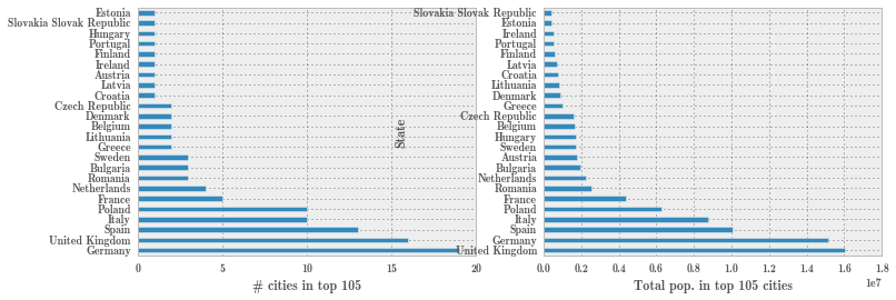
fig, (ax1, ax2) = plt.subplots(1, 2, figsize=(12, 4))

city_counts.plot(kind='barh', ax=ax1)
ax1.set_xlabel("# cities in top 105")
df_pop5.NumericPopulation.plot(kind='barh', ax=ax2)
ax2.set_xlabel("Total pop. in top 105 cities")
<matplotlib.text.Text at 0x7fd9e45f83d0>
时间序列
时间是个非常重要的维度,我们每时每刻都活在时间这个维度里,产生的数据也在时间这个维度里,所以时间可以拿来单独计算。
在 Python 环境下处理时间数据,如果不用 Pandas,就会用到 datetime,Pandas 中很多对时间序列的处理也是基于 datetime。
import datetime
先来建立一个关于时间序列的向量。
pd.date_range("2015-1-1", periods=31) # 时间起始点,时间长度,
DatetimeIndex(['2015-01-01', '2015-01-02', '2015-01-03', '2015-01-04',
               '2015-01-05', '2015-01-06', '2015-01-07', '2015-01-08',
               '2015-01-09', '2015-01-10', '2015-01-11', '2015-01-12',
               '2015-01-13', '2015-01-14', '2015-01-15', '2015-01-16',
               '2015-01-17', '2015-01-18', '2015-01-19', '2015-01-20',
               '2015-01-21', '2015-01-22', '2015-01-23', '2015-01-24',
               '2015-01-25', '2015-01-26', '2015-01-27', '2015-01-28',
               '2015-01-29', '2015-01-30', '2015-01-31'],
              dtype='datetime64[ns]', freq='D')
type(pd.date_range("2015-1-1", periods=31)) # DatetimeIndex
pandas.tseries.index.DatetimeIndex
dt = pd.date_range(datetime.datetime(2015, 1, 1), periods=31)
type(dt[1]) # 注意到时间向量的元素是时间戳格式的
pandas.tslib.Timestamp
pd.date_range(datetime.datetime(2015, 1, 1), periods=31) # 也可以使用 datetime 来创建
DatetimeIndex(['2015-01-01', '2015-01-02', '2015-01-03', '2015-01-04',
               '2015-01-05', '2015-01-06', '2015-01-07', '2015-01-08',
               '2015-01-09', '2015-01-10', '2015-01-11', '2015-01-12',
               '2015-01-13', '2015-01-14', '2015-01-15', '2015-01-16',
               '2015-01-17', '2015-01-18', '2015-01-19', '2015-01-20',
               '2015-01-21', '2015-01-22', '2015-01-23', '2015-01-24',
               '2015-01-25', '2015-01-26', '2015-01-27', '2015-01-28',
               '2015-01-29', '2015-01-30', '2015-01-31'],
              dtype='datetime64[ns]', freq='D')
pd.date_range("2015-1-1 00:00", "2015-1-1 12:00", freq="H") # 上面是按天,这里按小时,里面会把字符串格式转成时间格式
DatetimeIndex(['2015-01-01 00:00:00', '2015-01-01 01:00:00',
               '2015-01-01 02:00:00', '2015-01-01 03:00:00',
               '2015-01-01 04:00:00', '2015-01-01 05:00:00',
               '2015-01-01 06:00:00', '2015-01-01 07:00:00',
               '2015-01-01 08:00:00', '2015-01-01 09:00:00',
               '2015-01-01 10:00:00', '2015-01-01 11:00:00',
               '2015-01-01 12:00:00'],
              dtype='datetime64[ns]', freq='H')
上面是纯粹的时间向量,时间序列是以时间向量作为时间戳,作为 index,但数据还是实数值。index 是日期的 Series 是时间序列。
ts1 = pd.Series(np.arange(31), index=pd.date_range("2015-1-1", periods=31))
ts1.head() # index 是日期的被称为时间序列
2015-01-01    0
2015-01-02    1
2015-01-03    2
2015-01-04    3
2015-01-05    4
Freq: D, dtype: int64
ts1["2015-1-3"]
2
ts1.index[2]
Timestamp('2015-01-03 00:00:00', offset='D')
ts1.index[2].year, ts1.index[2].month, ts1.index[2].day # 可以取出对应的年月日
(2015, 1, 3)
type(ts1.index[2]) # 时间戳
pandas.tslib.Timestamp
ts1.index[2].to_pydatetime() # 可以转化成 datetime 基础的数据格式
datetime.datetime(2015, 1, 3, 0, 0)
上面介绍的是时间戳,还有一种时间数据是时间段,时间段和时间戳的区别在于,时间戳是个实点,时间段是个时间跨度。
periods = pd.PeriodIndex([pd.Period('2015-01'), pd.Period('2015-02'), pd.Period('2015-03')]) # 时间段,比如 2015-1 表示 2015 年 1 月之内
ts3 = pd.Series(np.random.rand(3), periods)
ts3
2015-01    0.036539
2015-02    0.472406
2015-03    0.036470
Freq: M, dtype: float64
type(periods[1]) # 时间段
pandas._period.Period
type(periods) # PeriodIndex
pandas.tseries.period.PeriodIndex
下面通过实例操练来学习时间序列的使用。
!head -n 5 temperature_outdoor_2014.tsv # 查看室外温度数据,时间和温度
1388530986	4.380000
1388531586	4.250000
1388532187	4.190000
1388532787	4.060000
1388533388	4.060000
!wc -l temperature_outdoor_2014.tsv # 看下该文件有多少行
49548 temperature_outdoor_2014.tsv
df1 = pd.read_csv('temperature_outdoor_2014.tsv', delimiter="	", names=["time", "outdoor"]) # tsv 和 csv 文件的区别在于,tsv 是以 tab 分隔符
df2 = pd.read_csv('temperature_indoor_2014.tsv', delimiter="	", names=["time", "indoor"])
df1.head() # 可以看到这里 time 并没有自动辨认为时间,而是以数值的形式
| time | outdoor | |
|---|---|---|
| 0 | 1388530986 | 4.38 |
| 1 | 1388531586 | 4.25 |
| 2 | 1388532187 | 4.19 |
| 3 | 1388532787 | 4.06 |
| 4 | 1388533388 | 4.06 |
df1.info() # 可以看到 time 是整数
<class 'pandas.core.frame.DataFrame'>
RangeIndex: 49548 entries, 0 to 49547
Data columns (total 2 columns):
time       49548 non-null int64
outdoor    49548 non-null float64
dtypes: float64(1), int64(1)
memory usage: 774.3 KB
这时要把 time 从数值转成时间。
df1.time = (pd.to_datetime(df1.time.values, unit="s")
              .tz_localize('UTC').tz_convert('Europe/Stockholm')) # 单位是秒,并设置时区
df1.info() # 可以看到 time 已经转成 datetime 格式
<class 'pandas.core.frame.DataFrame'>
RangeIndex: 49548 entries, 0 to 49547
Data columns (total 2 columns):
time       49548 non-null datetime64[ns, Europe/Stockholm]
outdoor    49548 non-null float64
dtypes: datetime64[ns, Europe/Stockholm](1), float64(1)
memory usage: 774.3 KB
type(df1.time[0]) # time 元素是时间戳
pandas.tslib.Timestamp
type(df1.time) # time 是序列
pandas.core.series.Series
df1 = df1.set_index("time") # 用时间来作为索引
df1.head()
| outdoor | |
|---|---|
| time | |
| 2014-01-01 00:03:06+01:00 | 4.38 |
| 2014-01-01 00:13:06+01:00 | 4.25 |
| 2014-01-01 00:23:07+01:00 | 4.19 |
| 2014-01-01 00:33:07+01:00 | 4.06 |
| 2014-01-01 00:43:08+01:00 | 4.06 |
df1.index[0] # time 元素是时间戳
Timestamp('2014-01-01 00:03:06+0100', tz='Europe/Stockholm')
type(df1.index) # time 设为 index 后,index 为 DatetimeIndex
pandas.tseries.index.DatetimeIndex
df2.time = (pd.to_datetime(df2.time.values, unit="s")
              .tz_localize('UTC').tz_convert('Europe/Stockholm'))
df2 = df2.set_index("time")
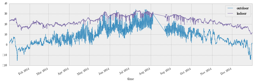
fig, ax = plt.subplots(1, 1, figsize=(12, 4)) # 把室内和室外温度画在一张图上,两个曲线叠加,横轴是时间,纵轴是温度
df1.plot(ax=ax);
df2.plot(ax=ax);

fig.tight_layout();
df1_jan = df1[(df1.index > "2014-1-1") & (df1.index < "2014-2-1")] # 选择子集,这种写法是比较繁琐的
df1_jan.head()
| outdoor | |
|---|---|
| time | |
| 2014-01-01 00:03:06+01:00 | 4.38 |
| 2014-01-01 00:13:06+01:00 | 4.25 |
| 2014-01-01 00:23:07+01:00 | 4.19 |
| 2014-01-01 00:33:07+01:00 | 4.06 |
| 2014-01-01 00:43:08+01:00 | 4.06 |
df1.index < "2014-2-1"
array([ True, True, True, ..., False, False, False], dtype=bool)
df2_jan = df2["2014-1-1":"2014-1-31"] # 这种选择子集的方式就很简洁,这里用冒号,跟之前用的 list 和 array 选择子集方式类似
上面是以每个数据点画图,下面把数据归结到月份来画图。这里介绍一种归结到月份的方式。
df_month = pd.concat([df.to_period("M").groupby(level=0).mean() for df in [df1, df2]], axis=1) # 对df1、df2 的index 只取月,做聚合对温度做平均
df_month.head(3) # 可以看到两列合并起来了,室外和室内的每月平均温度
| outdoor | indoor | |
|---|---|---|
| time | ||
| 2014-01 | -1.776646 | 19.862590 |
| 2014-02 | 2.231613 | 20.231507 |
| 2014-03 | 4.615437 | 19.597748 |
type(df_month)
pandas.core.frame.DataFrame
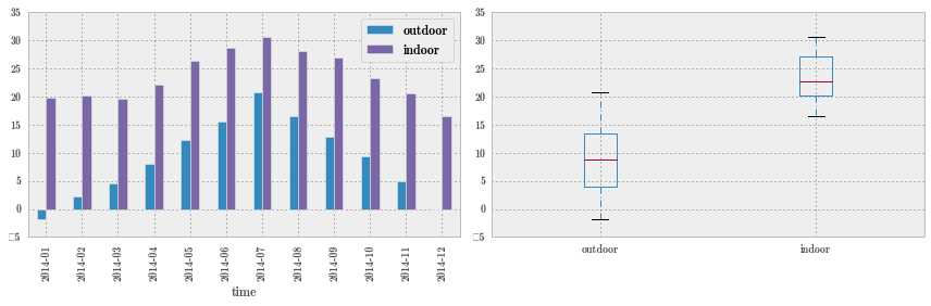
fig, axes = plt.subplots(1, 2, figsize=(12, 4))

df_month.plot(kind='bar', ax=axes[0]) # 如果有两列,自动画两个 bar,自动定义不同的颜色,非常方便
df_month.plot(kind='box', ax=axes[1]) # 箱线图

fig.tight_layout()
- 时间序列的应用场景有哪些?
分析金融和经济数据,也可用来分析服务器日志数据。
- 理解 DatatimeIndex 和 PeriodIndex 两种 Index 的差异,以及各自的创建方法。
DatatimeIndex 中的时间是实点,PeriodIndex 中的时间表示时间段。
dt = pd.date_range("2015-1-1", periods=31) # 创建 DatatimeIndex
print(type(dt))
print(dt)
<class 'pandas.tseries.index.DatetimeIndex'>
DatetimeIndex(['2015-01-01', '2015-01-02', '2015-01-03', '2015-01-04',
               '2015-01-05', '2015-01-06', '2015-01-07', '2015-01-08',
               '2015-01-09', '2015-01-10', '2015-01-11', '2015-01-12',
               '2015-01-13', '2015-01-14', '2015-01-15', '2015-01-16',
               '2015-01-17', '2015-01-18', '2015-01-19', '2015-01-20',
               '2015-01-21', '2015-01-22', '2015-01-23', '2015-01-24',
               '2015-01-25', '2015-01-26', '2015-01-27', '2015-01-28',
               '2015-01-29', '2015-01-30', '2015-01-31'],
              dtype='datetime64[ns]', freq='D')
pr = pd.PeriodIndex([pd.Period('2015-01'), pd.Period('2015-02'), pd.Period('2015-03')]) # 创建 PeriodIndex
print(type(pr))
print(pr)
<class 'pandas.tseries.period.PeriodIndex'>
PeriodIndex(['2015-01', '2015-02', '2015-03'], dtype='int64', freq='M')
补充阅读
- Pandas 官网
- 利用 Python 进行数据分析第 7、9、10 章
- Numerical Python第 12 章
- Data Preprocessing in Data Mining