Eddy Current Solver
• Solves sinusoidally-varying magnetic fields in frequency domain. Solves only for liner materials in 3D. It is a full wave solver thus considers displacement currents. Induced fields such as skin and proximity effects are also considered.
–涡流求解器
•解决频域中正弦变化的磁场。仅解决3D中的衬里材料。它是一个全波求解器,因此考虑位移电流。还考虑了感应场,例如趋肤和邻近效应。
【仿真介绍】
• Introduction to the Eddy Current Solver
– This workshop introduces the Eddy Current solver based on a simple example with a disk above a coil. This solver calculates the magnetic fields at a specified sinusoidal frequency. Both linear and nonlinear (for saturation effects) magnetic materials can be used. Also, eddy, skin and proximity effects are considered.
本仿真通过一个简单的线圈上带有一个磁盘(disk)的简单模型,介绍涡流解算器的使用。该计算器可以计算在特定频率正弦信号下的磁场。线性和非线性(饱和效应)的磁性材料均可以使用。此外,还考虑涡流,趋肤效应和邻近效应。
• 2D Geometry:
Iron Disk above a Spiral Coil – A sinusoidal 500 Hz current will be assigned to an eight turn spiral coil underneath of a cast iron disk. The coil induces eddy currents and losses in plate. The 2D model will be setup as shown below using the 2D RZ axisymmetric solver.
•2D几何:
螺旋线圈上方的铁盘–正弦500 Hz电流将分配给铸铁盘下面的八匝螺旋线圈。线圈在板中感应出涡流和损耗。如下所示,将使用2D RZ轴对称求解器建立2D模型。

【建模分析】
Step01 Create Design 创建设计文件
– Select the menu item Project -> Insert Maxwell 2D Design
Step02 Set Solution Type 设置解算器类型
– Select the menu item Maxwell 2D -> Solution Type
– Solution Type Window:
1. Geometry Mode: Cylindrical about Z
2. Choose Magnetic > Eddy Current
3. Click the OK button
如下图

Step03 Set Default Units 设置默认单位
– Select the menu item Modeler -> Units
• Set units to cm (centimeters) and press OK

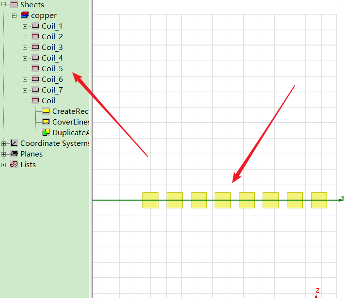
Step04 Create Coil 创建线圈
大小为一个2*2cm的矩形,对角线坐标为(17,0,-1)和(19,0,1),颜色设置为黄色,材料设置为铜
– Select the menu item Draw-> Rectangle
1. Using the coordinate entry fields, enter the position of rectangle
– X: 17, Y: 0, Z: -1, Press the Enter key
2. Using the coordinate entry fields, enter the opposite corner
– dX: 2, dY: 0, dZ: 2, Press the Enter key
– Change the name of resulting sheet to Coil and color to Yellow
– Change the material of the object to Copper
根据模型可知,需要8个相同的矩形模型,所以接下来将对该Coil进行复制操作,方法如下,每个矩形的中心距为3.1
共需要8个
Duplicate Coil
– Select the sheet Coil from history tree
– Select the menu item Edit-> Duplicate -> Along Line 线性排列
1. Using the coordinate entry fields, enter the first point of duplicate vector
– X: 0, Y: 0, Z: 0, Press the Enter key
2. Using the coordinate entry fields, enter the second point
– dX: 3.1, dY: 0, dZ: 0, Press the Enter key
• Total Number: 8
• Press OK
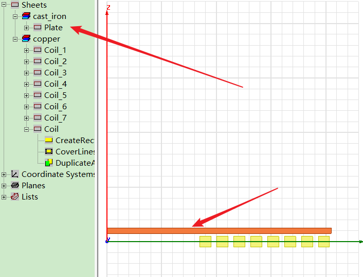
Step05 Create Plate 创建 plate
Plate的大小为41*1,顶点坐标为(0,0,1.5)和(41,0,2.5)材料为cast_iron铸铁,颜色为橘黄色
– Select the menu item Draw -> Rectangle
1. Using the coordinate entry fields, enter the position of rectangle
– X: 0, Y: 0, Z: 1.5, Press the Enter key
2. Using the coordinate entry fields, enter the opposite corner
– dX: 41, dY: 0, dZ: 1, Press the Enter key
– Change the name of resulting sheet to Plate and color to Orange
– Change the material of the object to cast_iron
Step06 Create Solution Region 创建解算区域
– Select the menu item Draw-> Rectangle
1. Using the coordinate entry fields, enter the position of rectangle
– X: 0, Y: 0, Z: -100, Press the Enter key
2. Using the coordinate entry fields, enter the opposite corner
– dX: 120, dY: 0, dZ: 200, Press the Enter key
– Change the name of resulting sheet to Region
Step07 Assign Excitations 创建激励
• Assign Excitation
– Press Ctrl and select all Coils from history tree
– Select the menu item Maxwell 2D -> Excitations -> Assign -> Current
– In Current Excitation window,
• Base Name: Current
• Value: 125 A
• Type: Solid
• Ref. Direction: Positive
• Press OK
注意:选择"Solid "指定将考虑线圈中的涡流效应。另一方面,如果选择"Stranded ",则仅会计算出直流电阻,而不会考虑线圈中的交流电影响。当趋肤深度比绞合导体的厚度大得多时,例如使用利兹线时,绞合是合适的。注意,在两种情况下,都将计算板中的涡流效应。
Step08 Assign Boundary and Parameters 创建边界和参数
• Assign Boundary
– Select the object Region from history tree
– Select the menu item Edit -> Select ->All Object Edges
– Select the menu item Maxwell 2D -> Boundaries -> Assign -> Balloon
– In Balloon Boundary window,
• Press OK
注意:在对称轴上,将自动跳过"气球边界"分配,这也可以通过选择不在对称轴上的区域的边缘来实现。
• Assign Matrix Parameters
– Select the menu item Maxwell 2D -> Parameters -> Assign -> Matrix
– In Matrix window,
• For all current Sources
– Include: þ Checked
• Press OK

Step09 Analyze 分析
• Create an analysis setup:
– Select the menu item Maxwell 2D -> Analysis Setup -> Add Solution Setup
– Solution Setup Window:
1. General Tab
– Maximum Number of Passes: 15
2. Solver Tab
– Adaptive Frequency: 500 Hz
3. Click the OK button
•Start the solution process:
1. Select the menu item Maxwell 2D -> Analyze All
Step10 Solution Data 结果数据
• View Solution Information
– Select the menu item Maxwell 2D -> Results -> Solution Data
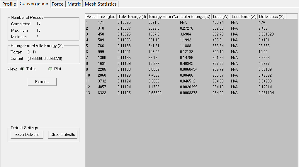
• To view Convergence
– Select the Convergence tab
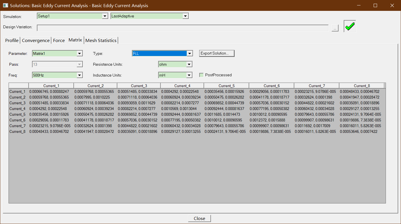
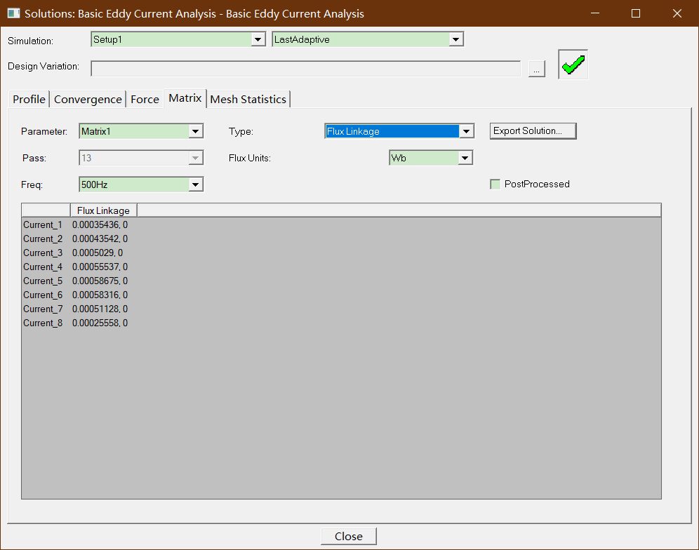
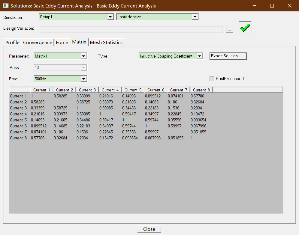
• To View Impedance matrix
– Select Matrix tab
– By default, the results are displayed as [R,Z] but can be also shown as [R,L] or as coupling coefficients.
Convergence:收敛性
阻抗矩阵

RL矩阵
Flux Linkage 磁链
Inductive Coupling Coefficient:电感耦合系数
Step11 Compute Power Loss 计算功率损耗
• Compute Total Power Loss in the Plate
– Select the menu item Maxwell 2D > Fields > Calculator
– In Fields Calculator window,
• Select Input > Quantity > OhmicLoss
• Select Input > Geometry
– Select Volume
– Select Plate
– Press OK
• Select Scalar > Integral > RZ
• Select Output > Eval

所以在Plate上的损耗大约是260W
Step12 Create Field Plots 创建场图
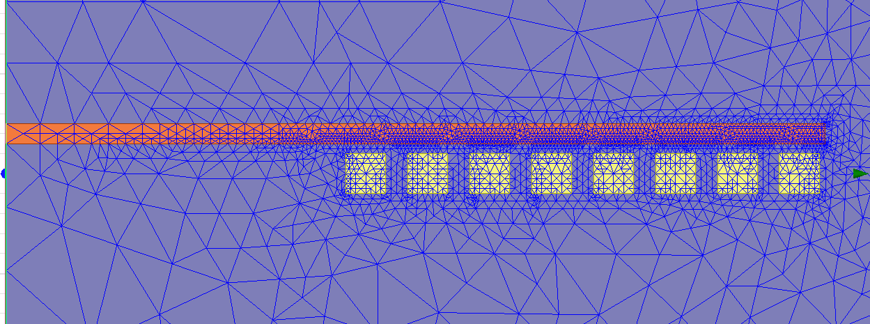
• Plot Mesh
– Select the menu item Edit > Select All
– Select the menu item Maxwell 2D > Fields > Plot Mesh
– In Create Mesh Plot window, press Done
• Plot Flux Lines
– Select the menu item Edit > Select All
– Select the menu item Maxwell 2D > Fields > Fields > A > Flux _Lines
– In Create Field Plot window, Press Done
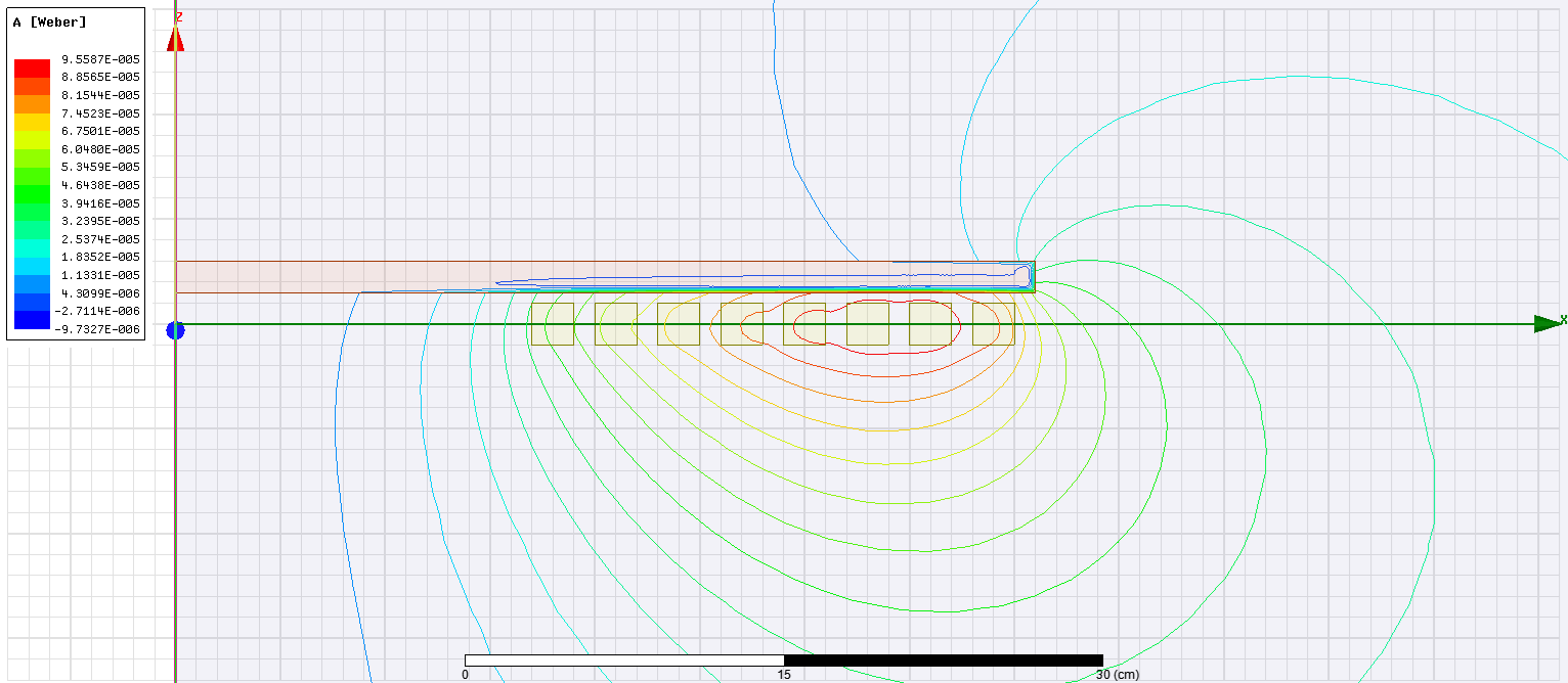
注意,由于磁力线是磁性的,因此磁力线被吸引到平板上。而且,由于板上有涡电流流动,因此在板上存在集肤效应。由图可以看出,极板上的磁力线分布不均匀,存在集肤效应
Step13 Create Field Plots (Contd…)
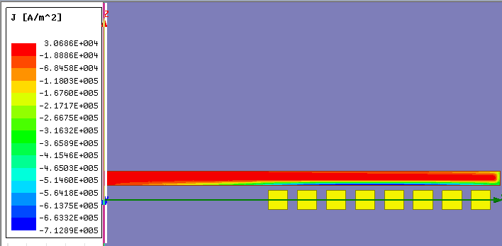
• Plot Current Density Scalar on Plate
– Select the sheet Plate from history tree
– Select the menu item Maxwell 2D Fields > Fields > J > JAtPhase
– In Create Field Plot window, Press Done
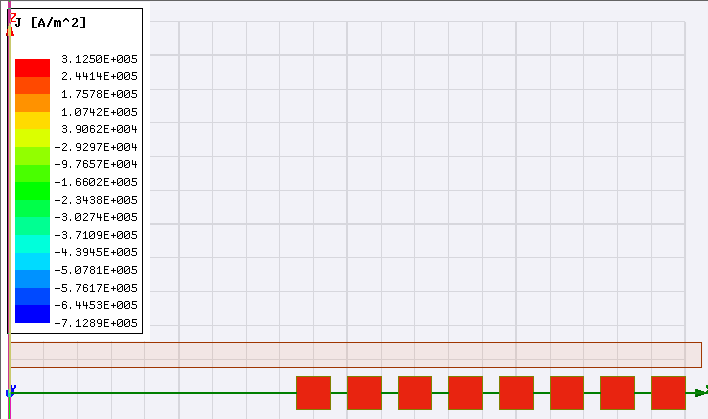
• Plot Current Density Scalar on Coils
– Press Ctrl and select all coils from history tree
– Select the menu item Maxwell 2D > Fields > Fields > J > JAtPhase
– In Create Field Plot window, Press Done
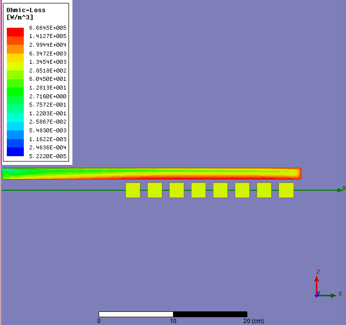
Step14 Plot Ohmic Loss Distribution
• Plot Ohmic Losses
– Press Ctrl and select all coils and Plate
– Select the menu item Maxwell 2D > Fields > Fields > Other > Ohmic_Loss
– In Create Field Plot window, Press Done
• Modify Plot Attributes
– Double click on the Legend to modify plot
– In the window,
• Scale tab
– Select Log
• Press Apply and Close
Step15 Plot Current Density Vectors
• Plot Current Density vectors
– Select the sheet Plate from history tree
– Select the menu item Maxwell 2D >Fields >Fields > J > J_Vector
– In Create Field Plot window, Press Done
– Double click on the Legend to modify plot
– In the window,
• Plots tab
– Plot: Change to J_Vector1
– Change Vector plot spacing
• Min: 0.5
• Max: 0.5
• Press Apply and Close
• Animate Plot
– Select the Vector plot from Project Manager tree, right click and select Animate
– In Setup Animation window,
• Press OK with default settings
– A window will appear to start, stop, pause or save the animation
Step16 将解算频率设置为1e-6Hz仿真DC情况下的情况
磁力线:
由图可以看出,在DC情况下,导体中的磁力线分布均匀,基本不存在集肤效应。
