深度学习和机器学习的区别
特征提取
- 机器学习的特征工程步骤是要靠手动完成的
- 深度学习通常由多个层组成,它们通常将更简单的模型组合在一起,将数据从一层传递到另一层来构建更复杂的模型。通过训练大量数据自动得出模型,不需要人工特征提取环节。
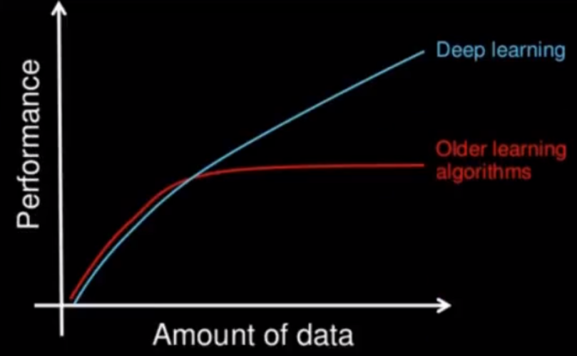
数据量和计算性能要求
机器学习需要的执行时间远少于深度学习,深度学习参数往往很庞大,需要通过大量数据的多次优化来训练参数。
算法代表
机器学习
朴素贝叶斯、决策树等
深度学习
神经网络
TensorFlow
结构
TensorFlow程序通常被组织成一个构建图阶段和一个执行图阶段。
在构建阶段,数据(张量Tensor)与操作(节点Op)的执行步骤被描述成一个图。
在执行阶段,使用会话执行构建好的图中的操作。
图和会话
- 图:这是TensorFlow将计算表示为指令之间的依赖关系的一种表示法
- 会话: TensorFlow跨一个或多个本地或远程设备运行数据流图的机制
张量
TensorFlow中的基本数据对象
节点
提供图当中执行的操作
图与TensorBoard
图结构
图包含了一组tf.Operation代表的计算单元对象和tf.Tensor代表的计算单元之间流动的数据。
图的相关操作
默认图
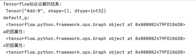
def tensorflow_demo():
    # Tensorflow实现加法
    a=tf.constant(2)
    b=tf.constant(3)
    #c=a+b(不提倡直接使用符合运算)
    c=tf.add(a,b)

    print("Tensorflow加法运算的结果:
",c)
    # 查看默认图
    # 方法1:调用方法
    default_g = tf.compat.v1.get_default_graph()
    print("default_g:
", default_g)
    # 方法2:查看属性
    print("a的图属性:
", a.graph)
    print("c的图属性:
", c.graph)
    #开启会话
    with tf.compat.v1.Session() as sess:
        c_t=sess.run(c)
        print("c_t:
",c_t)
        print("sess的图属性:
",sess.graph)

    return None
创建图
def create_graph():
    new_g = tf.Graph()
    with new_g.as_default():
        a_new = tf.constant(20)
        b_new = tf.constant(30)
        c_new = tf.add(a_new,b_new)
        print("c_new:
",c_new)
    #这时就不能用默认的sesstion了
    #开启new_g的会话
    with tf.compat.v1.Session(graph=new_g) as new_sess:
        c_new_value = new_sess.run(c_new)
        print("c_new_value:
",c_new_value)
        print("new_sess的图属性:
",new_sess.graph)
    return None

TensorBoard
数据序列化-events文件
TensorBoard 通过读取 TensorFlow 的事件文件来运行。TensorFlow 的事件文件包括了你会在 TensorFlow 运行中涉及到的主要数据。事件文件的生成通过在程序中指定tf.summary.FileWriter存储的目录,以及要运行的图
 # 1)将图写入本地生成events文件
        tf.compat.v1.summary.FileWriter("../tmp/summary", graph=new_sess.graph)
启动TensorBoard
tensorboard --logdir="summery"
![]()

OP
常见op

会话
一个运行TensorFlow operation的类。会话包含以下两种开启方式
- tf.Session:用于完整的程序当中
- tf.InteractiveSession:用于交互式上下文中的TensorFlow ,例如shell
target:如果将此参数留空(默认设置),会话将仅使用本地计算机中的设备。可以指定grpc://网址,以便指定TensorFlow 服务器的地址,这使得会话可以访问该服务器控制的计算机上的所有设备。
graph:默认情况下,新的tf.Session将绑定到当前的默认图。
config:此参数允许您指定一个tf.ConfigProto 以便控制会话的行为。例如,ConfigProto协议用于打印设备使用信息
run方法
run(fetches, feed_dict=None, options=None, run_metadata=None)
运行ops和计算tensor
- fetches 可以是单个图形元素,或任意嵌套列表,元组,namedtuple,dict或OrderedDict
- feed_dict 允许调用者覆盖图中指定张量的值
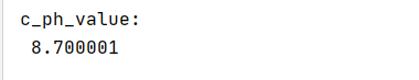
def session_demo():
    """
    会话的演示
    :return:
    """
    # 定义占位符
    a_ph = tf.compat.v1.placeholder(tf.float32)
    b_ph = tf.compat.v1.placeholder(tf.float32)
    c_ph = tf.add(a_ph, b_ph)

    # 开启会话
    with tf.compat.v1.Session(target='',graph=None,config=None) as sess:
        # 运行placeholder
        c_ph_value = sess.run(c_ph, feed_dict={a_ph: 3.9, b_ph: 4.8})
        print("c_ph_value:
", c_ph_value)

    return None
张量
TensorFlow的张量就是一个n维数组,类型为tf.Tensor。Tensor具有以下两个重要的属性
- type:数据类型
- shape:形状(阶)
阶
在TensorFlow系统中,张量的维数来被描述为阶.但是张量的阶和矩阵的阶并不是同一个概念.张量的阶(有时是关于如顺序或度数或者是n维)是张量维数的一个数量描述.
| 阶 | 数学实例 | Python | 例子 |
|---|---|---|---|
| 0 | 纯量 | (只有大小) | s = 483 |
| 1 | 向量 | (大小和方向) | v = [1.1, 2.2, 3.3] |
| 2 | 矩阵 | (数据表) | m = [[1, 2, 3], [4, 5, 6], [7, 8, 9]] |
| 3 | 3阶张量 | (数据立体) | t = [[[2], [4], [6]], [[8], [10], [12]], [[14], [16], [18]]] |
| n | n阶 | (自己想想看) | .... |
数据类型
| 数据类型 | Python 类型 | 描述 |
|---|---|---|
| DT_FLOAT | tf.float32 | 32 位浮点数. |
| DT_DOUBLE | tf.float64 | 64 位浮点数. |
| DT_INT64 | tf.int64 | 64 位有符号整型. |
| DT_INT32 | tf.int32 | 32 位有符号整型. |
| DT_INT16 | tf.int16 | 16 位有符号整型. |
| DT_INT8 | tf.int8 | 8 位有符号整型. |
| DT_UINT8 | tf.uint8 | 8 位无符号整型. |
| DT_STRING | tf.string | 可变长度的字节数组.每一个张量元素都是一个字节数组. |
| DT_BOOL | tf.bool | 布尔型. |
| DT_COMPLEX64 | tf.complex64 | 由两个32位浮点数组成的复数:实数和虚数. |
| DT_QINT32 | tf.qint32 | 用于量化Ops的32位有符号整型. |
| DT_QINT8 | tf.qint8 | 用于量化Ops的8位有符号整型. |
| DT_QUINT8 | tf.quint8 | 用于量化Ops的8位无符号整型. |
张量操作
tf.zeros(shape, dtype=tf.float32, name=None)
创建所有元素设置为零的张量。此操作返回一个dtype具有形状shape和所有元素设置为零的类型的张量。
tf.zeros_like(tensor, dtype=None, name=None)
给tensor定单张量(),此操作返回tensor与所有元素设置为零相同的类型和形状的张量。
tf.ones(shape, dtype=tf.float32, name=None)
创建一个所有元素设置为1的张量。此操作返回一个类型的张量,dtype形状shape和所有元素设置为1。
tf.ones_like(tensor, dtype=None, name=None)
给tensor定单张量(),此操作返回tensor与所有元素设置为1 相同的类型和形状的张量。
tf.fill(dims, value, name=None)
创建一个填充了标量值的张量。此操作创建一个张量的形状dims并填充它value。
tf.constant(value, dtype=None, shape=None, name='Const')
创建一个常数张量。
def tensor_demo():
    """
    张量的演示
    :return:
    """
    tensor1 = tf.constant(4.0)
    tensor2 = tf.constant([1, 2, 3, 4])
    linear_squares = tf.constant([[4], [9], [16], [25]], dtype=tf.int32)

    print("tensor1:
", tensor1)
    print("tensor2:
", tensor2)
    print("linear_squares_before:
", linear_squares)

    # 张量类型的修改
    l_cast = tf.cast(linear_squares, dtype=tf.float32)
    print("linear_squares_after:
", linear_squares)
    print("l_cast:
", l_cast)

    # 更新/改变静态形状
    # 定义占位符
    # 没有完全固定下来的静态形状
    a_p = tf.compat.v1.placeholder(dtype=tf.float32, shape=[None, None])
    b_p = tf.compat.v1.placeholder(dtype=tf.float32, shape=[None, 10])
    c_p = tf.compat.v1.placeholder(dtype=tf.float32, shape=[3, 2])
    print("a_p:
", a_p)
    print("b_p:
", b_p)
    print("c_p:
", c_p)
    # 更新形状未确定的部分
    # a_p.set_shape([2, 3])
    # b_p.set_shape([2, 10])
    # c_p.set_shape([2, 3])
    # 动态形状修改
    a_p_reshape = tf.reshape(a_p, shape=[2, 3, 1])
    print("a_p:
", a_p)
    # print("b_p:
", b_p)
    print("a_p_reshape:
", a_p_reshape)
    c_p_reshape = tf.reshape(c_p, shape=[2, 3])
    print("c_p:
", c_p)
    print("c_p_reshape:
", c_p_reshape)

    return None
变量op
def variable_demo():
    """
    变量的演示
    :return:
    """
    # 创建变量
    #修改变量的命名空间
    with tf.compat.v1.variable_scope("my_scope"):
        a = tf.Variable(initial_value=50)
        b = tf.Variable(initial_value=40)
    with tf.compat.v1.variable_scope("your_scope"):
        c = tf.add(a, b)
    print("a:
", a)
    print("b:
", b)
    print("c:
", c)

    # 初始化变量
    init = tf.compat.v1.global_variables_initializer()

    # 开启会话
    with tf.compat.v1.Session() as sess:
        # 运行初始化
        sess.run(init)
        a_value, b_value, c_value = sess.run([a, b, c])
        print("a_value:
", a_value)
        print("b_value:
", b_value)
        print("c_value:
", c_value)

    return None

案例:线性回归
原理回顾
根据数据建立回归模型,w1x1+w2x2+......b = y,通过真实值与预测值之间建立误差,使用梯度下降优化得到损失最小对应的权重和偏置。最终确定模型的权重和偏置参数。最后可以用这些参数进行预测。
- 构建模型:y = w1x1 + w2x2 + …… + wnxn + b
- 构造损失函数:均方误差
- 优化损失:梯度下降
API
运算
- 矩阵运算:tf.matmul(x, w)
- 平方:tf.square(error)
- 均值:tf.reduce_mean(error)
梯度下降优化
tf.train.GradientDescentOptimizer(learning_rate)
- learning_rate:学习率,一般为0~1之间比较小的值
- method:minimize(loss)
- return:梯度下降op
代码
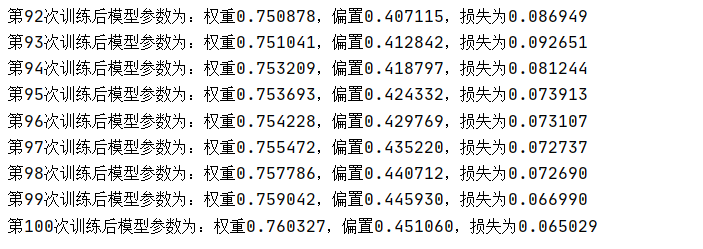
def linear_regression():
    """
    自实现一个线性回归
    :return:
    """
    # 1)准备数据
    X = tf.compat.v1.random_normal(shape=[100, 1])
    y_true = tf.matmul(X, [[0.8]]) + 0.7
    # 2)构造模型
    # 定义模型参数 用 变量
    weights = tf.Variable(initial_value=tf.compat.v1.random_normal(shape=[1, 1]))
    bias = tf.Variable(initial_value=tf.compat.v1.random_normal(shape=[1, 1]))
    y_predict = tf.matmul(X, weights) + bias
    # 3)构造损失函数
    error = tf.reduce_mean(tf.square(y_predict - y_true))
    # 4)优化损失
    optimizer = tf.compat.v1.train.GradientDescentOptimizer(learning_rate=0.01).minimize(error)
    # 显式地初始化变量
    init = tf.compat.v1.global_variables_initializer()
    # 开启会话
    with tf.compat.v1.Session() as sess:
        # 初始化变量
        sess.run(init)
        # 查看初始化模型参数之后的值
        print("训练前模型参数为:权重%f,偏置%f,损失为%f" % (weights.eval(), bias.eval(), error.eval()))
        #开始训练
        for i in range(100):
            sess.run(optimizer)
            print("第%d次训练后模型参数为:权重%f,偏置%f,损失为%f" % (i+1, weights.eval(), bias.eval(), error.eval()))

    return None