python - 3.7
pycharm
numpy-1.15.1
pandas-0.23.4
matplotlib-2.2.3
"""
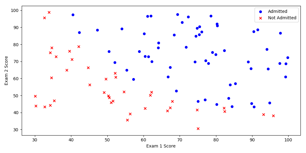
我们将建立一个逻辑回归模型来预测一个学生是否被大学录取。
假设你是一个大学系的管理员,你想根据两次考试的结果来决定每个申请人的录取机会。
你有以前的申请人的历史数据,你可以用它作为逻辑回归的训练集。
对于每一个培训例子,你有两个考试的申请人的分数和录取决定。
为了做到这一点,我们将建立一个分类模型,根据考试成绩估计入学概率。
时间:2018916 0016
"""
import numpy as np
import pandas as pd
import matplotlib.pyplot as plt
import os
pdData = pd.read_csv("LogiReg_data.txt", header = None, names = ["Exam 1", "Exam 2", "Admitted"])
print(pdData.head())
print(pdData.shape)
positive = pdData[pdData['Admitted'] == 1] # 指定
negative = pdData[pdData['Admitted'] == 0]
fig, ax = plt.subplots(figsize = (10, 5))
ax.scatter(positive["Exam 1"], positive["Exam 2"], s = 30, c = 'b', marker = 'o', label = "Admitted")
ax.scatter(negative["Exam 1"], negative["Exam 2"], s = 30, c = 'r', marker = 'x', label = "Not Admitted")
ax.legend()
ax.set_xlabel('Exam 1 Score')
ax.set_ylabel('Exam 2 Score')
plt.show()
运行结果:
D:Pythonpython.exe G:/编程/python/project/TYD/01/01/09/logireg_data.py
Exam 1 Exam 2 Admitted
0 34.623660 78.024693 0
1 30.286711 43.894998 0
2 35.847409 72.902198 0
3 60.182599 86.308552 1
4 79.032736 75.344376 1
(100, 3)
Process finished with exit code 0
"""
目标:
建立分类器(求解出三个参数 θ0,θ1,θ2) 为什么是3个参数,因为有一个偏置项
设定阈值,
根据阈值判断录取结果 #概率值
要完成的模块:
`sigmoid` : 映射到概率的函数
`model` : 返回预测结果值
`cost` : 根据参数计算损失
`gradient` : 计算每个参数的梯度方向
`descent` : 进行参数更新
`accuracy`: 计算精度
"""
"""
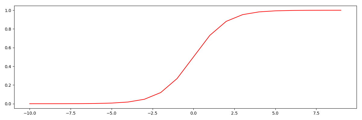
sigmoid函数 g(z)= 1/(1+e^(-z))
"""
def sigmoid(z): # 创建sigmoid函数
return 1 / (1 + np.exp(-z))
# 看看sigmoid函数长什么样
nums = np.arange(-10, 10, step = 1)
fig, ax = plt.subplots(figsize = (12, 4))
ax.plot(nums, sigmoid(nums), 'r')
plt.show()
"""
    g:R→[0,1]
    g(0) = 0.5
    g(-∞) = 0
    g(+∞) = 1
"""
运行结果:
pdData.insert(0, 'Ones', 1)  # 插入偏置列
orig_data = pdData.as_matrix()
#print(orig_data.shape)
#print(orig_data.shape[1])
cols = orig_data.shape[1]  # 取列数
X = orig_data[:, 0:cols - 1]  # 切片[行1:行N,列1:列N],取X的矩阵
Y = orig_data[:, cols - 1:cols]
theta = np.zeros([1, 3])  # 构建θ矩阵,1行3列,相当于构建3个θ参数
print('
')
print(X[0:5])
print('
')
print(Y[0:5])
print('
')
print(theta)
运行结果:
[[ 1. 34.62365962 78.02469282]
[ 1. 30.28671077 43.89499752]
[ 1. 35.84740877 72.90219803]
[ 1. 60.18259939 86.3085521 ]
[ 1. 79.03273605 75.34437644]]
[[0.]
[0.]
[0.]
[1.]
[1.]]
[[0. 0. 0.]]
"""
    损失函数:D(hθ(x),y) = -ylog(hθ(x))-(1-y)log(1-hθ(x))
    平均损失值:J(θ) = 1/n求和1-n:(D(hθ(x),y))
    -ylog(hθ(x))一部分
    (1-y)log(1-hθ(x))一部分
"""


def cost(X, Y, theta):
    left = np.multiply(-Y, np.log(model(X, theta)))
    right = np.multiply(1 - Y, np.log(1 - model(X, theta)))
    return np.sum(left - right) / len(X)  # J(θ)


test_cost = cost(X, Y, theta)
print("
", test_cost)
运行结果:
0.6931471805599453