Chapter 5 Getting Started with pandas
这一章要介绍 pandas 的基础。
都是数据处理包,pandas 和 numpy 的区别在于:
While pandas adopts many coding idioms from NumPy, the biggest difference is that pandas is designed for working with tabular or heterogeneous data. NumPy, by contrast, is best suited for working with homogeneous numerical array data.
也就是说,pandas 更适合列成表的 (tabular) 或者是多种类的 (heterogeneous) 数据,而 numpy 更适合同种类的 (homogeneous) 数据。
让我们开始吧!
Introduction to pandas Data Structures
pandas 中两类最常用的数据结构就是 Series 和 DataFrame。
Series
Series 是类似于一维 ndarray 的对象,包括一组值和每个值的索引,有点像 dict ,最简单的形式如下:
obj = pd.Series([1,2,3,4])
print(obj)
# Out:
# 0    1
# 1    2
# 2    3
# 3    4
# dtype: int64
使用 values 和 index 可以查看 obj 的值和索引。
不指定 Series 的索引是类似可以默认为 range(0,n+1),也可以指定 index ,会按照指定的顺序排列 index。
obj2 = pd.Series([4, 7, -5, 3], index=['d', 'b', 'a', 'c'])
Series 的一些方法和 numpy 的 ndarray 是很类似的:
# call by index
obj2['a']
obj2[['a','b','c']]
# boolean index
obj2[obj2 > 0]
# functions
obj2 * 2
np.exp(obj2)

# dict like 这里要用 index 判断
'b' in obj2
Series 还可以通过 dict 创建,以及规定 keys 创建:
sdata = {'Ohio': 35000, 'Texas': 71000, 'Oregon': 16000, 'Utah': 5000}
states = ['California', 'Ohio', 'Oregon', 'Texas']
obj4 = pd.Series(sdata, index=states)
print(obj4)
# California        NaN
# Ohio          35000.0
# Oregon        16000.0
# Texas         71000.0
# dtype: float64
可以使用 pd.isnull() 或 pd.notnull() 确定是否存在缺失的数据。
Series 的 value 和 index 都拥有 name 属性。
Series 的 index 可以通过赋值语句修改。但是不能单独修改其中某一个 index,例如 obj.index[1] = 's' 就是不可以的。TypeError: Index does not support mutable operations
obj = pd.Series([1,2,3,4])
obj.index = ['a','b','c','d']
DataFrame
A DataFrame represents a rectangular table of data and contains an ordered collection of columns, each of which can be a different value type (numeric, string, boolean, etc.).
DataFrame 类似可以理解为是一张 excel 表,也可以认为是一个共享 index 的 Series 的 dict。
data = {'state': ['Ohio', 'Ohio', 'Ohio', 'Nevada', 'Nevada', 'Nevada'],
        'year': [2000, 2001, 2002, 2001, 2002, 2003],
        'pop': [1.5, 1.7, 3.6, 2.4, 2.9, 3.2]}
frame = pd.DataFrame(data)
head方法可以展示前五行的数据;也可以在定义的时候通过 column 参数调整顺序,通过 index 调整 index 的值。
调用的时候可以使用 dict-like 的方法,也可以使用属性的方法:
frame['year']
frame.year
获取 year 后返回的 Series 与 DataFrame 有着相同的 index。
可以使用loc()获取 DataFrame 的某一行。
DataFrame 的某一列也可以通过赋值(包括标量或者数组)的方式修改;也可以通过 Series 给 DataFrame 的某一列赋值:
data = {'state': ['Ohio', 'Ohio', 'Ohio', 'Nevada', 'Nevada', 'Nevada'],
        'year': [2000, 2001, 2002, 2001, 2002, 2003],
        'pop': [1.5, 1.7, 3.6, 2.4, 2.9, 3.2]}
frame = pd.DataFrame(data, columns=['year', 'state', 'pop', 'debt'])
debt = pd.Series([-1.2,-1.5,-3.4], index=[1,4,2])
frame.debt = debt
print(frame)
新增一列就直接给赋值即可;del 方法可以通过列名称删除某一列。
如果使用 nested dict 创建 DataFrame 时,dict 的 outer key 作为 column name,inner key 作为 index。
pop = {'Nevada': {2001: 2.4, 2002: 2.9},
        'Ohio': {2000: 1.5, 2001: 1.7, 2002: 3.6}}
frame = pd.DataFrame(pop)
print(pop)
#          Nevada  Ohio
# 2000     NaN   1.5
# 2001     2.4   1.7
# 2002     2.9   3.6
pd.DataFrame(index)的优先级高于 nested dict 的内键,即如果参数 index 与内键不一致,那么以 index 参数为准。
pop = {'Nevada': {2001: 2.4, 2002: 2.9},
        'Ohio': {2000: 1.5, 2001: 1.7, 2002: 3.6}}
pop = pd.DataFrame(pop, index=[0,1,2])
print(pop)
#    Nevada  Ohio
# 0     NaN   NaN
# 1     NaN   NaN
# 2     NaN   NaN
dict of Series 也是这样:
pop = {'Nevada': {2001: 2.4, 2002: 2.9},
        'Ohio': {2000: 1.5, 2001: 1.7, 2002: 3.6}}
pop = pd.DataFrame(pop)
pdata = {'Ohio': pop['Ohio'][:-1], 'Nevada': pop['Nevada'][:2]}
print(pd.DataFrame(pdata))
DataFrame 的 index 和 column 都有 name 属性,可以通过赋值改变。
DataFrame 的 values 属性包括全部的数据,dtype 会选择一个可以包括全部数据类型的对象。
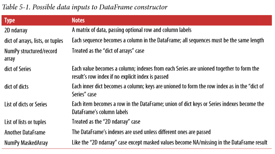
可以接受的用于创建 DataFrame 的数据类型:
Index Objects
Index objects are immutable and thus can’t be modified by the user. Immutability makes it safer to share Index objects among data structures.
DataFrame 的 columns 和 index 都是 pd.Index Object,同时:
Unlike Python sets, a pandas Index can contain duplicate labels.
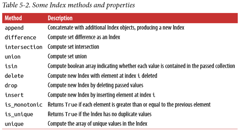
一些注意事项:
append的参数是pd.Index,不是 list 或一些 array-like 类型;difference表示 A - B,用法是A.difference(B);drop只可以用在 unique value 的 Index 中,否则会报 InvalidIndexError;insert只可以在 i 处插入一个值,index.insert(1, [2,3,4,10])这种写法是不允许的;is_unique和is_monotonic都是属性,不是方法。
Essential Functionality
Reindexing
虽然可以通过对 index 赋值实现 index 的修改,但是对应的数值并不会改变,所以 reindex 方法就是干这个事的。reindex的详细文档
其中 method 参数规定了集中补全 gap 的形式:
- ffill:从前向后补齐,用当前最近的有效值补全无效值;
- bfill:从后向前补齐;
- nearest:从后向前,用第一次遇到的有效值补齐目前所有遇到的无效值。
也可以 reindex columns: DataFrame.reindex(columns=[])
Dropping Entries from an Axis
简单来说就是从 index 和 columns 两个维度删数据,index:DataFrame.drop([index_name]), columns: DataFrame.drop([columns_name], axis=1)。
还可以通过 inplace 参数设置是否原地修改。
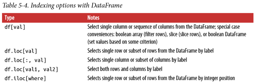
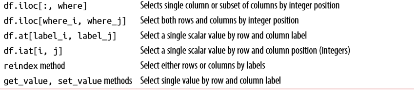
Indexing, Selection, and Filtering
之前讲过的什么 slicing,boolean indexing 技巧啥的在这里都可以用,还是既可以从 index 维度又可以从 columns 上用来选择符合的数据。另外,index 还可以用整数下表来代替。
还有就是通过 loc 或者 iloc 访问某一行,loc 是用 index_name,iloc 使用整数(integer)代替 index_name,也可以在得到一行后用 columns_name 来过滤数据。
下表是通过 index 获取数据的一些办法:
Arithmetic and Data Alignment
主要介绍了 Series 在进行算术运算时的处理过程,如果两个 Series 中都存在的 index,相应的数值相加,否则引入 missing。
在 DataFrame 中也是一样,只有在 index 和 columns 都相同时才能进行算术运算。极端情况是如果两个 DataFrame 中没有相交的 index,那么算术运算之后的 DataFrame 就全是 Nan。
Arithmetic methods with fill values
根据上一节,当一个位置出现 Nan 时,两个 Series 或者 DataFrame 相应位置的算数运算结果就是 Nan,但如果想做 overlap 的操作(实在是不知道怎么描述这种情况hhh),就需要 fill_value 这个属性。
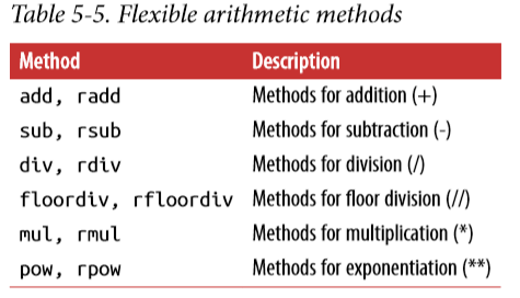
See Table 5-5 for a listing of Series and DataFrame methods for arithmetic. Each of them has a counterpart, starting with the letter r, that has arguments flipped. So these two statements are equivalent:
1 / df1
df1.rdiv(1)
Operations between DataFrame and Series
pandas 定义了 DataFrame 和 Series 的计算,其中涉及 broadcasting 的知识。
需要注意的是,axis=0 或 axis='index' 表示在 index 维度上进行运算,直观上来理解就是竖着算:
frame = pd.DataFrame(np.arange(12.).reshape((4, 3)),
        columns=list('bde'),index=['Utah', 'Ohio', 'Texas', 'Oregon'])

series = frame['d']
print(frame)
print(frame.sub(series, axis=0))
# Out:
#           b     d     e
# Utah    0.0   1.0   2.0
# Ohio    3.0   4.0   5.0
# Texas   6.0   7.0   8.0
# Oregon  9.0  10.0  11.0
#           b    d    e
# Utah   -1.0  0.0  1.0
# Ohio   -1.0  0.0  1.0
# Texas  -1.0  0.0  1.0
# Oregon -1.0  0.0  1.0
Function Application and Mapping
之前提到的 numpy ufunc 对 DataFrame 和 Series 也是适用的。
对于自定义的函数,可以使用 apply 方法:
f = lambda x: x.max() - x.min()
# 默认 axis=0
frame.apply(f)
frame.apply(f, axis=1)
apply 是以 DataFrame 的每个行或列为对象的,applymap 是以 DataFrame 的每个元素作为对象的。下面这段代码展示了这两个方法的区别:
frame = pd.DataFrame(np.random.randn(4, 3),
        columns=list('bde'),index=['Utah', 'Ohio', 'Texas', 'Oregon'])
format = lambda x: '%.2f' % x
print(frame.applymap(format))

for col in frame.columns:
        frame[col] = frame[col].apply(format)
        # frame[col] = frame[col].map(format)
print(frame)
Sorting and Ranking
sort_index 方法对 index 进行排序,通过设置参数 axis 来决定是排 index(0) 还是 column(1),设置参数 ascending 来决定排序顺序,True 是升序,False 是降序。
sort_values 方法对 value 进行排序,设置参数 by 决定是按照哪一列的顺序来排,如果有两个以上的 column_name,意思就是在前一个值相同的时候,按照下一列的降序来排列:
frame = pd.DataFrame({'b': [4, 7, -3, 2], 'a': [0, 1, 0, 1]})
frame.sort_values(by=['a', 'b'])
#    a  b
# 2  0 -3
# 0  0  4
# 3  1  2
# 1  1  7
Ranking 也就是对 Series 或 DataFrame 中的行或列进行排名,通过 method 参数的不同会有不同的 rank 方式。rank的官方文档,顺便吐槽一下我自己的英文水平,看到 rank 一直想的是矩阵的秩。。。
Axis Indexes with Duplicate Labels
因为 index 允许重复,所以当通过 index_name 获取重复 index 的值时,会取出相同 index_name 的所有行。
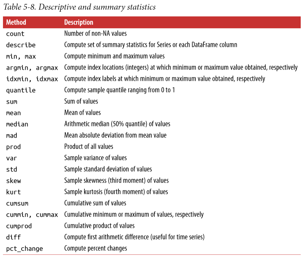
Summarizing and Computing Descriptive Statistics
numpy 中的简单统计方法在 Series 和 DataFrame 中都可以使用。
还有一些方法可以简单地提供一些统计量:
Correlation and Covariance
A.corr(B) 计算两个 Series 的相关系数;
A.cov(B) 计算两个 Series 的协方差;
df.corr(), df.cov() 计算一个相关系数(协方差)矩阵;
df.corrwith() 计算 df 与 选择的行或列之间的相关系数;
Unique Values, Value Counts, and Membership
series.value_counts() 计算元素个数;
series.isin([]) 计算 series 中是否存在所说的元素,返回一个 boolean series;
series.unique() 返回 series 中 unique 的元素 series;
Conclusion
In the next chapter, we’ll discuss tools for reading (or loading) and writing datasets with pandas. After that, we’ll dig deeper into data cleaning, wrangling, analysis, and visualization tools using pandas.