Isolation Forest Implementation（孤立森林）

Isolation Forest Implementation

Isolation Forest Implementation

Isolation Forest Learning!

服务于异常检测（Services for anomaly detection )

iForest 适用于连续数据(Discrete vs Continuous)的anomaly detection.

Q1 why iForest are suitable for continuous data ?

Since we are only interested in continuous valued attributes in this paper, all nominal and binary attributes are removed. （From the paper)

在 iForest 中异常被定义为 “容易被孤立的离群点(more likely to be separated)”

(Anomalies are defined in iForest as "outliers that are more likely to be separated.")

异常点一般都是非常稀有的，在iTree中会很快被划分到叶子节点，因此可以用叶子节点到根节点的路径 h(x) 长度来判断一条记录x是否是异常点。（Assumption1. 可以理解为iForest的原理）

Q2: can u speak some others anomaly definitions?

Passage From 机器之心

异常检测是对不符合预期模式或数据集中其他项目的项目，事件和观测值的识别，异常有时候也被称之为离群值，新奇，噪声，偏差和例外。

可以理解为分布稀疏且离密度高的群体较远的点。（有点类似Kmeas）

(can be interpreted as points that are sparsely distributed and distant from the high density population)

算法设计的主要流程分为三个大步骤：

1. iTree 的设计

既然算法中明确说了 Forest ，iTree 则是组成Forest的结构。

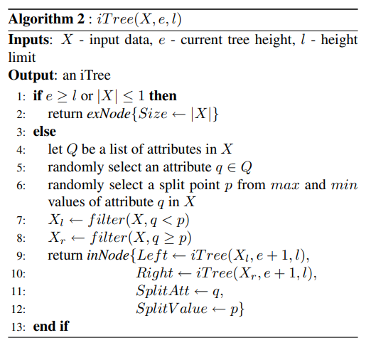
构建 iTree 的伪代码如上所示，用我的理解就是：

iTree 是一颗由随机二叉树，每个非叶子结点都有一个属性和值，我们称之为splitAtt 和 splitVal 用于将数据集进行划分。对于每个叶子结点其形成有两种可能：

第一种是树的高度已经达到了预设的高度 height_limit

第二种是当前数据集 (X) 的大小已经小于等于 (1)。

这里有几个疑问：

为什么要预设高度以及如何预设高度？

根据 iTree 如何判断是否为异常？

2. iForest 的构建

这里首先我们需要理解 bagging methods ，我们可以简单理解为不断有放回抽样一部分然后用抽样出来的数据集 (X^prime) 进行 iTree 的训练。

伪代码如上，我们首先根据样本的大小设置iTree的最大深度，然后我们根据给定的 (t) 随机构建相应数量的 iTree。

既然我们需要随机的抽取样本，那么样本大小 (psi) 我们如何确定呢？

根据论文里说的（同时也是区别于 Random Forest），随机采集的数据样本大小 (psi) 不需要等于 (n) 样本大小，而是可以远小于 (n) 论文中提到当 (psi > 256) 时效果的提升就不大了。

An analysis on the effect sub-sampling size can be found in section 5.2 which shows that the detection performance is near optimal at this default setting and insensitive to a wide range of (psi).

——《Isolation Forest》

同时还有一个公式没有被我们解释：

[l(verb|height_limit|) = lceil log_2psi ceil ]

这是由于根据前文中的 Assumption.1 ，我们认为异常的点在iTree中位于的深度很浅，而 (l(verb|height_limit|) = lceil log_2psi ceil) 是将高度限制为平均值之内，在异常检测中我们只对那些路径长度短于平均水平的数据点感兴趣。

Note that the tree height limit (l) is automatically set by the sub-sampling size (psi): (l = ceiling(log_2 psi)), which is approximately the average tree height [7]. The rationale of growing trees up to the average tree height is that we are only interested in data points that have shorter-than average path lengths, as those points are more likely to be anomalies.

——《Isolation Forest》

但是这样处理之后，由于存在高度限制，因此有些结点可能还没有划分就结束并停留在叶子上，也就是说：他们在树中的深度(h(x))应该比当前的更深，因此在后文计算每个结点(x_i)在某一棵 iTree 中的深度时，会在结尾处增加一个trick .

3. 评判异常

根据上文的描述，我们判断一个结点是否为异常结点的主要依据是他在iTree中的深度。

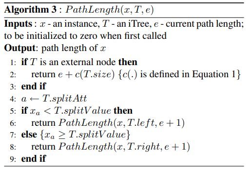
该算法的伪代码如上，可以发现其过程大体与在BST中搜索某个结点类似，但是在抵达external node也就是叶子时，有一个(c(T.size))，我们首先不管 (c) 是什么公式，这里之所以要做修正是因为我们在前面限制了height_limit因此我们在这里要根据这团簇的数量对评分做一个补偿。

现在就到了最终的部分，how to check the anomaly node ，一个在中国博客中很少有人比较细致分析的部分：

首先我们重新提一遍Assumption.1: 异常点一般都是非常稀有的，在iTree中会很快被划分到叶子节点，因此可以用叶子节点到根节点的路径 h(x) 长度来判断一条记录x是否是异常点。

我们会发现一个情况，iTree和BST的结构很像，那我们可以借助BST的结论：the average path length of unsuccessful search in BST as:【BST的失败查找等于这里查找到根结点】

[c(n) = 2H(n-1) - 2(n-1)/n ]

其中 (H(i)) 是调和级数可以写为：(H(i) = ln(i)+gamma|gamma =0.577215... 欧拉常数)。既然(c(n))是(h(n))的均值，那么我们可以用他来对(h(n))进行正则化，联立Assumption.1我们将异常评分定义为：

[s(x, psi) = 2^{-dfrac{E(h(x))}{c(psi)}} ]

这样定义，会出现3种情况：

when (E(h(x)) ightarrow c(n), s ightarrow 0.5)
when (E(h(x)) ightarrow 0, s ightarrow 1)
when (E(h(x)) ightarrow n-1, s ightarrow 1)

这也是为什么可以通过这个公式(s(x, psi))得出是否异常。

优缺点

iForest具有线性时间复杂度。因为是ensemble的方法，所以可以用在含有海量数据的数据集上面。通常树的数量越多，算法越稳定。由于每棵树都是互相独立生成的，因此可以部署在大规模分布式系统上来加速运算。
什么是 ensemble 方法？

首先这里介绍了什么是集成方法：Ensemble methods

可以简单理解为：把几种机器学习的算法组合到一起，或者把同一种算法的不同参数组合到一起。

主要分为如下两类：
1. Averaging methods （平均方法）就是利用训练数据的全集或者一部分数据训练出几个算法或者一个算法的几个参数，最终的算法是所有这些算法的算术平均。比如Bagging Methods（装袋算法），Forest of Randomized Trees（随机森林）等
2. Boosting methods（提升算法），就是利用一个基础算法进行预测，然后在后续的其他算法中利用前面算法的结果，重点处理错误数据，从而不断的减少错误率。其动机是使用几种简单的弱算法来达到很强大的组合算法。所谓提升就是把“弱学习算法”提升(boost)为“强学习算法，是一个逐步提升逐步学习的过程；某种程度上说，和neural network有些相似性。经典算法比如AdaBoost（Adaptive Boost，自适应提升），Gradient Tree Boosting（GBDT）。PS:这个我有时间再强化一下
关于 Bagging(装袋法) link，注意就是一种有放回的抽样方法来生成训练数据 可以并行。

这里我们需要搞清楚，Isolation Forest 和 Randomized Trees 之间的区别

RF

随机森林是有监督算法！IForest是无监督
iForest不适用于特别高维的数据。由于每次切数据空间都是随机选取一个维度，建完树后仍然有大量的维度信息没有被使用，导致算法可靠性降低。高维空间还可能存在大量噪音维度或无关维度（irrelevant attributes），影响树的构建。
iForest仅对Global Anomaly 敏感，即全局稀疏点敏感，不擅长处理局部的相对稀疏点（Local Anomaly）。

异常检测的对比

一些算法的介绍：

PCA [10]

MCD: Minimum Covariance Determinant [11, 12]

OCSVM: One-Class Support Vector Machines [3]

LOF: Local Outlier Factor [1]

kNN: k Nearest Neighbors [19, 20]

HBOS: Histogram-based Outlier Score [5]

FastABOD: Fast Angle-Based Outlier Detection using approximation [7]

Isolation Forest [2]

Feature Bagging [9]

效果：

总体来看，没有任何模型表现持续最好。Isolation Forest和KNN的表现非常稳定，分别在ROC和PRN上有比较优秀的表现。

KNN等模型基于距离度量，因此受到数据维度的影响比较大，当维度比较低时表现很好。如果异常特征隐藏在少数维度上时，KNN和LOF类的效果就不会太好，此时该选择Isolation Forest。

部分模型较不稳定，受到数据变化的影响较大，如HBOS在8个数据上表现优异，但也在3个数据上变现最差。

简单模型的表现不一定差，比如KNN和MCD的原理都不复杂，但表现均不错。

ABOD综合来看效果最差，应该避免。这个实验中所用的ABOD版本是FastABOD并用10个近邻进行近似，可能精准版的ABOD效果会好一些，但运算复杂度会大幅度上升((O(n^3)))。

From [知乎--异常检测](数据挖掘中常见的「异常检测」算法有哪些？ - 微调的回答 - 知乎 https://www.zhihu.com/question/280696035/answer/417091151)

Q&A：

Q1：异常检测的评价标准和指标有什么？

Q2：关于LOF，KNN的学习？

代码实现

其中我们数据集使用的是：

Kaggle credit card fraud competition data set

关于该数据集的介绍

The dataset contains transactions made by credit cards in September 2013 by European cardholders.

This dataset presents transactions that occurred in two days, where we have 492 frauds out of 284,807 transactions. The dataset is highly unbalanced, the positive class (frauds) account for 0.172% of all transactions.

It contains only numerical input variables which are the result of a PCA transformation. Unfortunately, due to confidentiality issues, we cannot provide the original features and more background information about the data. Features V1, V2, … V28 are the principal components obtained with PCA, the only features which have not been transformed with PCA are 'Time' and 'Amount'. Feature 'Time' contains the seconds elapsed between each transaction and the first transaction in the dataset. The feature 'Amount' is the transaction Amount, this feature can be used for example-dependant cost-sensitive learning. Feature 'Class' is the response variable and it takes value 1 in case of fraud and 0 otherwise.

Given the class imbalance ratio, we recommend measuring the accuracy using the Area Under the Precision-Recall Curve (AUPRC). Confusion matrix accuracy is not meaningful for unbalanced classification.

该数据集包含欧洲持卡人在2013年9月通过信用卡进行的交易。

这个数据集呈现了两天内发生的交易，在284,807笔交易中，我们有492笔欺诈。该数据集是高度不平衡的，正面类（欺诈）占所有交易的0.172%。

它只包含数字输入变量，是PCA转换的结果。不幸的是，由于保密问题，我们不能提供原始特征和关于数据的更多背景信息。特征V1, V2, ... V8是用PCA得到的主成分，唯一没有经过PCA转换的特征是时间和金额。特征'时间'包含每笔交易与数据集中第一笔交易之间的秒数。特征Amount是交易金额，这个特征可用于依赖实例的成本敏感型学习。特征Class是响应变量，在欺诈的情况下取值为1，否则为0。

# -*- coding: utf-8 -*-
"""
Created on Sat Sep 18 00:22:12 2021

@author: 文柯力
"""
import numpy as np
import pandas as pd
def C(psi):
    """
    异常分数
    anomaly score 
    why C? 为什么用这个公式呢？
    """
    H = lambda _psi: np.log(_psi) + 0.5772156649
    if psi > 2:
        return 2 * H(psi - 1) - 2 * (psi - 1) / psi
    elif psi == 2:
        return 1
    return 0

class LeafNode:
    """ 叶子 """
    def __init__(self, size, data):
        # services for pathLength calculate below. 
        self.size = size
        self.data = data

class DecisionNode:
    """ split node  """
    def __init__(self, left, right, splitAtt, splitVal):
        self.left = left
        self.right = right
        self.splitAtt = splitAtt
        self.splitVal = splitVal

class iTree:
    def __init__(self, height, height_limit):
        self.height = height
        self.height_limit = height_limit
    
    def fit(self, X: np.ndarray):
        if self.height >= self.height_limit or X.shape[0] <= 1:
            self.root = LeafNode(X.shape[0], X)
            return self.root 
        # Choose Random Split Attributes and Value 
        num_features = X.shape[1]
        # Note the high is exclusive
        splitAtt = np.random.randint(0, num_features)
        splitVal = np.random.uniform(min(X[:, splitAtt]), max(X[:, splitAtt]))
        
        # Make X_left and X_right
        X_left  = X[X[:, splitAtt] <  splitVal]
        X_right = X[X[:, splitAtt] >= splitVal]
        
        left  = iTree(self.height + 1, self.height_limit)
        right = iTree(self.height + 1, self.height_limit)
        left.fit(X_left)
        right.fit(X_right)
        
        self.root = DecisionNode(left.root, right.root, splitAtt, splitVal)
        # i don't know why we need to count it 
        # self.n_nodes = self.count_nodes(self.root)
        return self.root 
    
        
    
class IsolationTreeEnsemble:
    def __init__(self, sample_size = 256, n_trees = 10):
        self.sample_size = sample_size
        self.n_trees = n_trees
    def fit(self, X: np.ndarray):
        """
        Given a 2D matrix of observations, creat an ensemble of IsolationTree objects
        and store them in a list: self.trees. Convert DataFrames to ndarray objects.
        """
        self.trees = []
        if isinstance(X, pd.DataFrame):
            X = X.values
        n_rows = X.shape[0]
        height_limit = np.ceil(np.log2(self.sample_size))   
        
        for i in range(self.n_trees):
            # using Bagging methods. 
            # do u think about that if smaple_size greater than n_rows ?
            data_index = np.random.randint(0, n_rows, self.sample_size)
            X_sub = X[data_index]
            # print(X_sub)
            tree = iTree(0, height_limit)
            tree.fit(X_sub)
            self.trees.append(tree)
        
        # allow chaning 
        return self
    
    def PathLength(self, X: np.ndarray) -> np.ndarray:
        """
        Given a 2D matrix of observations, X, compute the average path length
        for each observation in X.  
        Compute the path length for x_i using every tree in self.trees then 
        compute the average for each x_i.  Return an ndarray of shape (len(X),1).
        """
        paths = []
        for row in X:
            avg_path, cnt = 0, 0
            for tree in self.trees:
                node = tree.root
                cur_length = 0
                while isinstance(node, DecisionNode):
                    if (row[node.splitAtt] < node.splitVal):
                        node = node.left
                    else:
                        node = node.right 
                    cur_length += 1
                
                # The adjustment(`C(leaf_size)`) accounts for an unbuilt
                # subtree beyond the tree height limit. 
                leaf_size = node.size
                pathLength = cur_length + C(leaf_size)
                
                # dynamic updates the average pathLength 
                avg_path = (avg_path * cnt + pathLength) / (cnt + 1)
                cnt += 1
            paths.append(avg_path)

        return np.array(paths)
    
    def anomaly_score(self, X:pd.DataFrame) -> np.ndarray:
        """
        Given a 2D matrix of observations, X, compute the 
        anomaly score for each x_i observaton, returning an 
        ndarry of them.
        """
        if isinstance(X, pd.DataFrame):
            X = X.values
        avg_length = self.PathLength(X)
        scores = np.array([np.power(2, -ech / C(self.sample_size)) for ech in avg_length])
        return scores
    
    def predict(self, X: np.ndarray, threshold=0.5):
        """
        Givend an 2D matrix of observations, X 
        using anomaly_score() to calculate scores and 
        return an array of prediction: 1 for any score >= threshold and 0 otherwise.
        u can see that the default value of threshold is 0.5 
        """
        scores = self.anomaly_score(X)
        prediction = np.array(
            [1 if s >= threshold else 0 for s in scores]
        )
        return prediction