梯度下降（三）

梯度下降法可以进行一些优化以加快运行速度：

一，对数据源进行特征缩放

二，把批量梯度下降改为随机梯度下降或者小批量梯度下降

数据源（包括训练集的输入，训练集的输出，初始设置的超参数theta，预测集的输入）

import numpy as np
import random

X = np.array([[425.5, 8.12, 17.5],
              [422.3, 8.32, 22.9],
              [418.0, 8.36, 23.7],
              [419.2, 8.20, 21.1],
              [384.2, 8.86, 23.3],
              [372.5, 7.70, 19.1],
              [372.9, 8.46, 18.2],
              [380.8, 8.88, 22.2],
              [401.7, 9.00, 27.6],
              [406.5, 8.80, 28.8],
              [410.5, 9.26, 27.8]])

Y = np.array([7.450, 7.605, 7.855, 7.805, 6.900,
              7.470, 7.385, 7.225, 8.130, 8.720, 9.145])

init_theta = np.array([0.0, 0.0, 0.0, 0.0])

Prediction_set = np.array([[390.0, 8.00, 20.0],
                           [391.6, 7.96, 23.6],
                           [403.5, 9.01, 25.9]])

梯度下降函数

相比上一节中的梯度下降函数，这里的函数多了一个参数batch，当batch等于训练集中样本个数时，该函数等价于上一节的批量梯度下降函数，当batch=1时，该函数为随机梯度下降函数，当batch介于两者之间时，即为小批量梯度下降函数，当训练集样本数量很大时，选择一个合适的批量可以有效降低训练时间。

def gradient_descent(X, Y, theta, batch, max_iter=10000, learning_rate=0.01):

    # 数据预处理
    X = np.insert(X, 0, values=1, axis=1)
    Y = np.mat(Y).T
    theta = np.mat(theta).T

    # 常量定义
    sample_size = len(X)
    sample_list = range(0, sample_size)

    # 梯度下降主体
    for i in range(max_iter):

        # 随机选择batch个样本作为本轮梯度下降的标准
        # 使用sample生成的x和y是样本乱序的，但是样本的乱序不会影响theta的更新
        selected_sample = random.sample(sample_list, batch)
        x = X[selected_sample, :]
        y = Y[selected_sample, :]

        # 更新theta参数
        theta -= (learning_rate / batch) * x.T * (x * theta - y)

    # 检验迭代完成时代价函数的值
    cost = np.sum(np.asarray(X * theta - Y) ** 2) / sample_size
    print("Cost =", cost)

    # 返回训练好的参数theta
    return theta

数据的标准化和预测

在使用梯度下降之前，可以对训练集和预测集进行特征缩放

常用的特征缩放有归一化和标准化等。

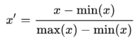
归一化

标准化

预测集以及其结果必须要用同样的数据进行缩放最后才能得到正确的结果。

# 数据标准化(利用了numpy中的广播机制)
X_mean = X.mean(axis=0)
X_std = X.std(axis=0)
Y_mean = Y.mean()
Y_std = Y.std()

X = (X - X_mean) / X_std
Y = (Y - Y_mean) / Y_std

theta = gradient_descent(X, Y, init_theta, 5, learning_rate=0.001)

Prediction_set = (Prediction_set - X_mean) / X_std
Prediction_set = np.insert(Prediction_set, 0, values=1, axis=1)

result = Prediction_set * theta
result = result * Y_std + Y_mean
print(result)

输出结果

cost可以反应训练拟合的好坏程度

Cost = 0.3990182552092087
[[7.40042959]
 [7.85839981]
 [8.11422701]]

为了简化代码，文中用了一定numpy中的处理方法，比如matrix和ndarray的转换以及广播机制等，在numpy常见用法一文中再详细写。