=================第2周 神经网络基础===============
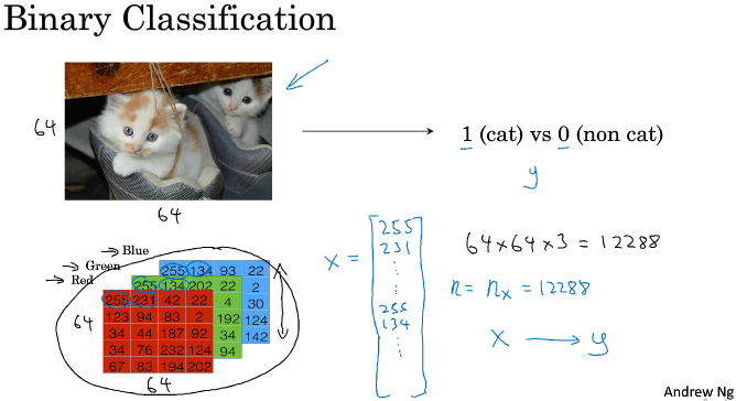
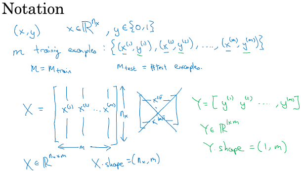
===2.1 二分分类===
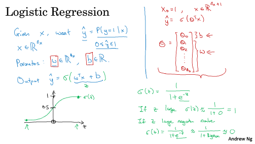
===2.2 logistic 回归===
It turns out, when you implement you implement your neural network, it will be easier to just keep b and w as separate parameters. 本课程中将分开考虑它们。
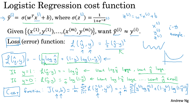
===2.3 logistic 回归损失函数===
损失函数loss func是在单个样本上定义的,而代价函数cost func它衡量在全体训练样本上的表现。其实Logistic Model 可以被看作是 一个非常小的神经网络。
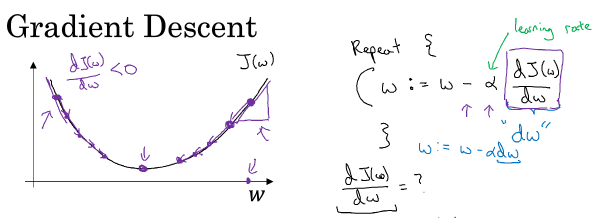
===2.4 梯度下降法===
凸函数这性质是我们使用logistic回归的这个特定成本函数J的重要原因之一。通常用0来初始化<w, b>,其他初始化也ok。
仔细体会下图,梯度,梯度的正负,负梯度才是下降方向。也体会下,如果某点的梯度为正,那w增大,J也会增大。
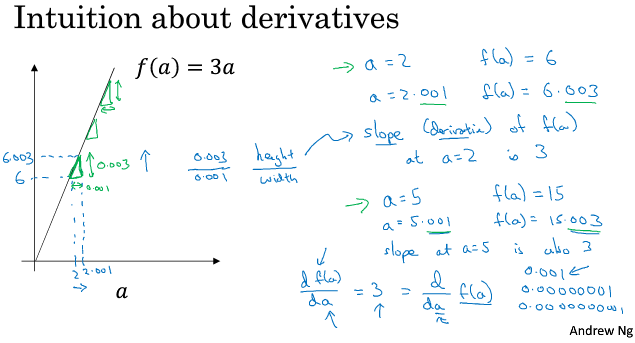
===2.5 导数===
一个直观的理解是,delta_y的变化是 delta_x 的变化的 dy/dx 倍。导数的定义是你右移a 一个不可度量的无限小的值, f(a)会增加 df/da times a的改变值。
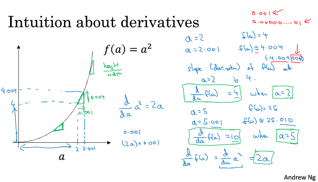
===2.6 更多导数的例子===
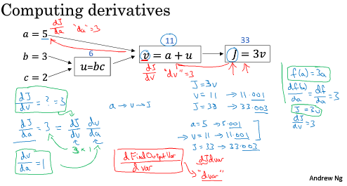
===2.7 计算图=== &
===2.8 计算图的导数计算===
仔细体会一下,求导的链式法则,当a改变0.001时,J改变多少,a是如何影响J的。
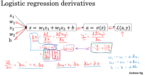
===2.9 logistic 回归中的梯度下降法===
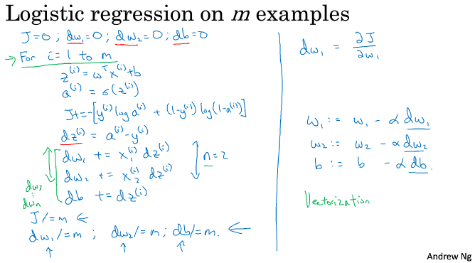
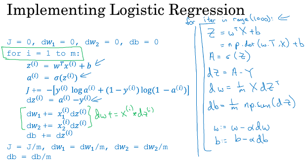
===2.10 m 个样本的梯度下降===
m个样本的梯度下降的逐样本迭代版本。当你应用深度算法时,你会发现在代码中显式地使用for循环会使算法很低效。
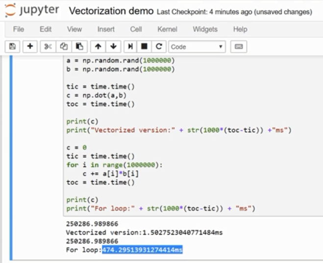
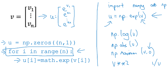
===2.11 向量化===
下面的比较可以看出,向量化了之后快了大概 300 倍。
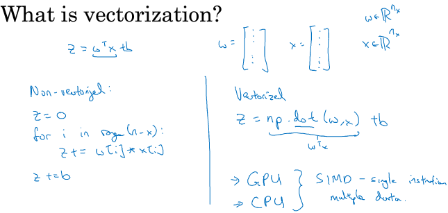
GPU和CPU都有并行化的指令,有时候会叫做SIMD指令(single instruction multiple data.),意思是如果你使用了这样的内置函数np.function or other functions that don't require you explicitly implementing a for loop. It enables Python numpy to take much better advantage of parallelism. 这点对GPU和CPU上面计算都是成立的,GPU非常擅长SIMD计算,but CPU is actually also not too bad at that. 经验法则是 只要有其他可能 就不要使用显式for循环。
===2.12 向量化的更多例子===
尝试用numpy内置函数代替显示loop实现你想要的功能。
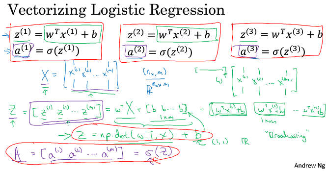
===2.13 向量化 logistic 回归===
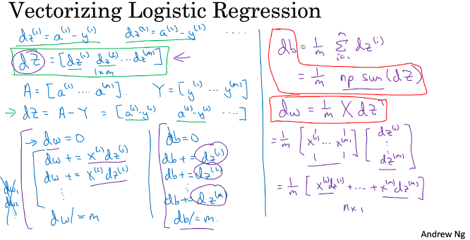
===2.14 向量化 logistic 回归的梯度输出===
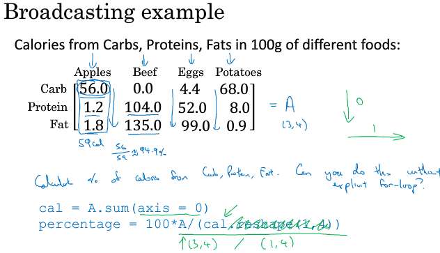
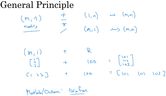
===2.15 Python 中的广播===
Broadcasting。例子中的 cal 后面的 reshape 其实可以不用加,但当我编写Python代码时,if I'm not entirely sure what matrix, whether the dimensions of a matrix, 我会经常调用reshape命令 确保它是正确的列向量或行向量。
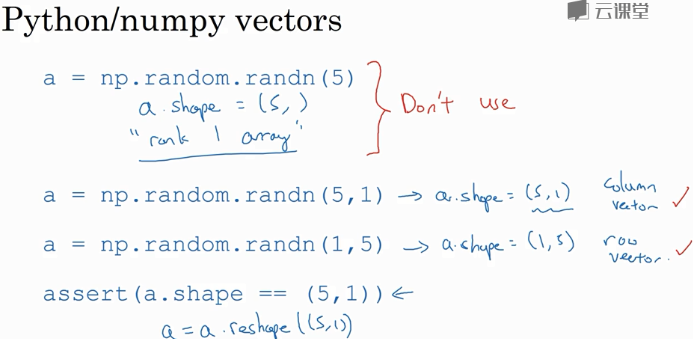
===2.16 关于 python / numpy 向量的说明===
注意在 In[7] 的这个数据结构中 有2个方括号,之前只有1个,So that's the difference between this is really a 1 by 5 matrix versus one of these rank 1 arrays.
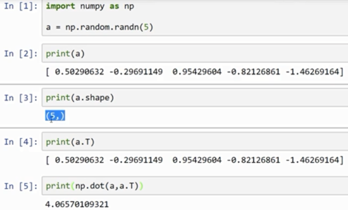
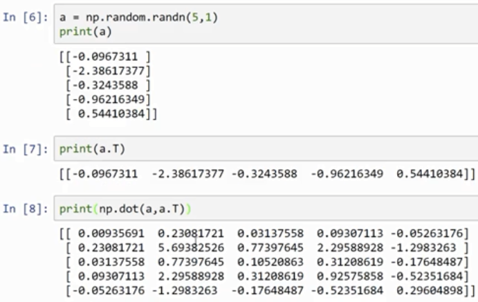
rank 1 array 的行为和行向量或列向量都不一样,which makes some of its effects nonintuitive. 我的建议是不要使用它们。如果某些时候确实得到了rank 1 array,你可以用reshape,使它的行为更好预测。
===2.17 Jupyter / Ipython 笔记本的快速指南===
使用愉快:)
===2.18 (选修)logistic代价函数的推导===
If you assume that the training examples I've drawn independently or drawn IID, then the probability of the example is the product of probabilities. 从1到m的 p(y^(i) |x^(i))的概率乘积。