之前在kaggle上做了关于房价预测的比赛,现整理如下。
解决问题的大概步骤是:
1、通过画图查看目标变量SalePrice是否偏分布,若是,则进行log(x+1)变换。并查看数值变量,若偏度大于0.75,也做log(x+1)变换
2、缺失值处理。分类变量NA NA值赋值为0,数值变量中的NA赋值为其平均值
3、将分类变量转化为哑变量
4、回归分析。分别用Ridge回归与Lasso回归进行回归分析,因为Lasso回归的误差平均值更小,所以选取Lasso回归的结果作为最终预测结果
具体代码如下:
library(ggplot2)
library(plyr)
library(dplyr)
library(caret)
library(moments)
library(glmnet)
library(elasticnet)
library(knitr)
train=read.csv("train.csv",stringsAsFactors = F,header = T)
test=read.csv("test.csv",stringsAsFactors = F,header = T)
all_data=rbind(select(train,MSSubClass:SaleCondition),select(test,MSSubClass:SaleCondition))
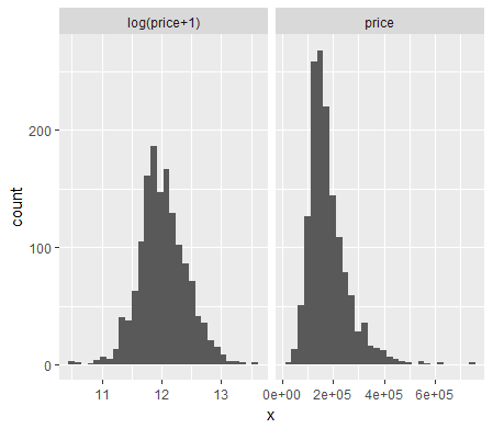
#画出售价的直方图,发现左偏,用log(x+1)进行调整
df=rbind(data.frame(version="log(price+1)",x=log(train$SalePrice+1)),data.frame(version="price",x=train$SalePrice))
ggplot(data=df)+facet_wrap(~version,ncol=2,scales="free_x")+geom_histogram(aes(x=x))
train$SalePrice=log(train$SalePrice+1)
#数值变量偏度》0.75时做log变换
feature_classes <- sapply(names(all_data),function(x){class(all_data[[x]])})
numeric_feats <-names(feature_classes[feature_classes != "character"])
skewed_feats <- sapply(numeric_feats,function(x){skewness(all_data[[x]],na.rm=TRUE)})
skewed_feats <- skewed_feats[skewed_feats > 0.75]
for(x in names(skewed_feats)) {
all_data[[x]] <- log(all_data[[x]] + 1)
}
#分类变量,dummy variables
categorical_feats <- names(feature_classes[feature_classes == "character"])
dummies <- dummyVars(~.,all_data[categorical_feats])
categorical_1_hot <- predict(dummies,all_data[categorical_feats])
categorical_1_hot[is.na(categorical_1_hot)] <- 0
#数值变量,用平均值弥补缺失值
numeric_df <- all_data[numeric_feats]
for (x in numeric_feats) {
mean_value <- mean(train[[x]],na.rm = TRUE)
all_data[[x]][is.na(all_data[[x]])] <- mean_value
}
#预处理后的重建data
all_data <- cbind(all_data[numeric_feats],categorical_1_hot)
X_train <- all_data[1:nrow(train),]
X_test <- all_data[(nrow(train)+1):nrow(all_data),]
y <- train$SalePrice
#models
CARET.TRAIN.CTRL <- trainControl(method="repeatedcv",
number=5,
repeats=5,
verboseIter=FALSE)
lambdas <- seq(1,0,-0.001)
set.seed(123) # for reproducibility
model_ridge <- train(x=X_train,y=y,
method="glmnet",
metric="RMSE",
maximize=FALSE,
trControl=CARET.TRAIN.CTRL,
tuneGrid=expand.grid(alpha=0, # Ridge regression
lambda=lambdas))
ggplot(data=filter(model_ridge$result,RMSE<0.14)) +
geom_line(aes(x=lambda,y=RMSE))
mean(model_ridge$resample$RMSE)
# [1] 0.1308965
set.seed(123) # for reproducibility
model_lasso <- train(x=X_train,y=y,
method="glmnet",
metric="RMSE",
maximize=FALSE,
trControl=CARET.TRAIN.CTRL,
tuneGrid=expand.grid(alpha=1, # Lasso regression
lambda=c(1,0.1,0.05,0.01,seq(0.009,0.001,-0.001),
0.00075,0.0005,0.0001)))
model_lasso
mean(model_lasso$resample$RMSE)
# [1] 0.1260769
coef <- data.frame(coef.name = dimnames(coef(model_lasso$finalModel,s=model_lasso$bestTune$lambda))[[1]],
coef.value = matrix(coef(model_lasso$finalModel,s=model_lasso$bestTune$lambda)))
coef <- coef[-1,]
picked_features <- nrow(filter(coef,coef.value!=0))
not_picked_features <- nrow(filter(coef,coef.value==0))
cat("Lasso picked",picked_features,"variables and eliminated the other",
not_picked_features,"variables
")
coef <- arrange(coef,-coef.value)
imp_coef <- rbind(head(coef,10),
tail(coef,10))
ggplot(imp_coef) +
geom_bar(aes(x=reorder(coef.name,coef.value),y=coef.value),
stat="identity") +
ylim(-1.5,0.6) +
coord_flip() +
ggtitle("Coefficents in the Lasso Model") +
theme(axis.title=element_blank())
preds <- exp(predict(model_lasso,newdata=X_test)) - 1
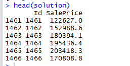
solution <- data.frame(Id=as.integer(rownames(X_test)),SalePrice=preds)
write.csv(solution," lasso_sol.csv",row.names=FALSE)
预测结果如下:
其他的尝试:
尝试将lasso和ridge方法的预测结果,按照权重相加得到最终预测结果,但是结果并不理想,还没有单独lasso的效果好。可能跟设置的权重有关系,但在这个问题上本来ridge的方法就没有lasso好,权重相加本身可能就拉低了lasso预测效果。
听闻XGBoost在此方面效果比较好,或可一试。