背景:MNIST 数据集来自美国国家标准与技术研究所,National Institute of Standardsand Technology (NIST).
数据集由来自250个不同人手写的数字构成,其中50%是高中学生,50%来自人口普查局(the Census Bureau)的工作人员
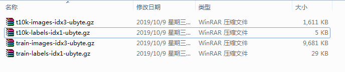
其中,训练集55000验证集5000 测试集10000。MNIST 数据集可在 http://yann.lecun.com/exdb/mnist/ 获取,也可以不下载因为TensorFlow提供了数据集读取方法。
一、数据下载和读取
1.1数据下载
import tensorflow as tf
import tensorflow.examples.tutorials.mnist.input_data as input_data
mnist = input_data.read_data_sets("MNIST_data/",one_hot=True)
MNIST数据集文件在读取时如果指定目录下不存在,则会自动去下载,需等待一定时间如果已经存在了,则直接读取。
1.2数据读取
import tensorflow.examples.tutorials.mnist.input_data as input_data

mnist = input_data.read_data_sets("MNIST_data/",one_hot=True)
print('训练集train 数量:',mnist.train.num_examples,',验证集 validation 数量:',mnist.validation.num_examples,',测试集test 数量:',mnist.test.num_examples)

print('train images shape:',mnist.train.images.shape,'labels shaple:',mnist.train.labels.shape)
#(55000,784)意思是5w5千条,每一条784位(图片大小28*28);(55000,10):10分类 One Hot编码

1.2.1数据的批量读取
MNIST数据包里提供了 .next_batch方法,可实现批量读取

1.3可视化image
def plot_image(image):
      plt.imshow(image.reshape(28,28),cmap='binary')
      plt.show()
plot_image(mnist.train.images[1])

二、标签数据与独热编码
2.1独热编码简介
一种稀疏向量,其中:一个元素设为1,所有其他元素均设为0
独热编码常用于表示拥有有限个可能值的字符串或标识符
例如:假设某个植物学数据集记录了15000个不同的物种,其中每个物种都用独一无二的字符串标识符来表示。在特征工程过程中,可能需要将这些字符串标识符编码为独热向量,向量的大小为15000
为什么要采用one hot编码?
- 将离散特征的取值扩展到了欧式空间,离散特征的某个取值就对应欧式空间的某个点
- 机器学习算法中,特征之间距离的计算或相似度的常用计算方法都是基于欧式空间的
- 将离散型特征使用one-hot编码,会让特征之间的距离计算更加合理
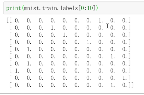
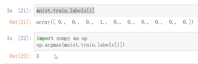
独热编码如何取值?
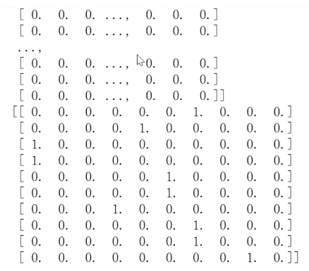
非独热编码的标签值:

三、模型构建
3.1定义待输入数据的占位符
#mnist 中每张图片共有28*28=784个像素点
x=tf.placeholder(tf.float32,[None,784],name="X")
#0-9一共10个数字=>10个类别
y=tf.placeholder(tf.float32,[None,10],name="Y")
3.2定义模型变量
在本案例中,以正态分布的随机数初始化权重W,以常数0初始化偏置b
W= tf.Variable(tf.random_normal([784,10]),name="W")
b= tf.Variable(tf.zeros([10]),name="b")
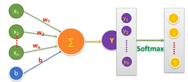
3.3定义前向计算和结果分类
forward = tf.matmul(x, W) + b #前向计算
当我们处理多分类任务时,通常需要使用Softmax Regression模型。
Softmax Regression会对每一类别估算出一个概率。
工作原理:将判定为某一类的特征相加,然后将这些特征转化为判定是这一类的概率。
pred = tf.nn.softmax(forward) #Softmax分类
四、训练模型
4.1设置训练参数
train_epochs = 50   #训练轮数
batch_size=100      #单次训练样本数(批次大小)
total_batch= int(mnist.train.num_examples/batch_size)#一轮训练有多少批次
display_step=1     #显示粒度
learning_rate=0.01   #学习率
4.2定义损失函数,选择优化器
loss_function = tf.reduce_mean(-tf.reduce_sum(y*tf.log(pred),reduction_indices=1))   #定义交叉熵损失函数
optimizer = tf.train.GradientDescentOptimizer(learning_rate).minimize(loss_function)  #梯度下降优化器
4.3定义准确率
#检查预测类别tf.argmax(pred,1)与实际类别tf.argmax(y.1)的匹配情况,argmax能把最大值的下标取出来
correct_prediction = tf.equal(tf.argmax(pred,1),tf.argmax(y,1))#相等则返回True
#准确率,将布尔值转化为浮点数,并计算平均值
accuracy = tf.reduce_mean(tf.cast(correct_prediction,tf.float32))
sess = tf.Session()#声明会活
init = tf.global_variables_initializer()#变量初始化
sess.run(init)
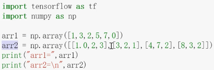
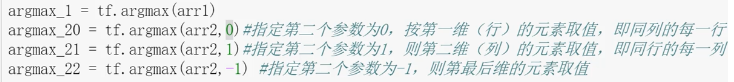
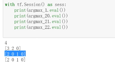
拓展部分:argmax()用法

4.4训练过程
#开始训练
for epoch in range(train_epochs):
    for batch in range(total_batch):
          xs,ys = mnist.train.next_batch(batch_size)  # 读取批次数据
          sess.run(optimizer,feed_dict={x:xs,y:ys})   # 执行批次训练
    #total_batch个批次训练完成后,使用验证数据计算课差与准确率;验证集没有分批
    loss,acc = sess.run([loss_function,accuracy],feed_dict={x:mnist.validation.images,y:mnist.validation.labels})
    #打印训练过程中的详细信息
    if (epoch+1) % display_step == 0:
        print("Train Epoch:",'%02d' %(epoch+1),"Loss=","{:.9f}".format(loss),"Accuracy=","{:.4f}".format(acc))
print("Train Finished!")
运行结果为:
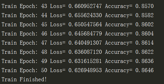
从结果可以看出,损失值Loss是趋于更小的,准确率Accuracy越来越高,可以修改参数,使得准确率(验证集)到90%以上~~
五、评估模型
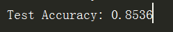
完成训练后,在测试集上评估模型的准确率
accu_test = sess.run(accuracy,feed_dict={x:mnist.test.images,y:mnist.test.labels})
print("Test Accuracy:",accu_test)
Note:测试环节中没有分批,所有测试数据1万条直接执行

测试结果86.14%, 上面模型训练时是由验证集的数据做出来的,是86.46%。
在训练集上评估模型的准确率
accu_train = sess.run(accuracy,feed_dict={x:mnist.train.images,y:mnist.train.labels})
print("Test Accuracy:",accu_train)
通过数据集的合理划分,训练和验证效果差不多,准确率比较满意则可以进行模型预测。
六、模型应用和可视化
#模型预测
#由于pred预测结果是one-hot编码格式,所以需要转换为0-9数字
prediction_result = sess.run(tf.argmax(pred,1),feed_dict={x:mnist.test.images})

print(prediction_result[0:10])  #查看预测结果中的前10项
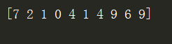
然而不够直观,不能与数据集的图片相对应。
6.1定义可视化函数
 1 def plot_images_labels_prediction(images,labels,prediction,index,num=10):   #图像列表,标签列表,预测值列表,从第index个开始显示 , 缺省一次显示10幅
 2     fig = plt.gcf() #获取当前图表,get current figure
 3     fig.set_size_inches(10,12)  #1英寸等于2.54cm
 4     if num > 25:
 5         num = 25  #最多显示25个子图
 6     for i in range(0, num):
 7         ax = plt.subplot(5,5,i+1)  #获取当前要处理的子图
 8         ax.imshow(np.reshape(images[index], (28, 28)),cmap='binary')  # 显示第index个图像
 9         title = "label=" + str(np.argmax(labels[index]))# 构建该图上要显示的
10         if len(prediction)>0:
11             title += ",predict="+ str(prediction[index])
12         ax.set_title(title, fontsize=10)  #显示图上title信息
13         ax.set_xticks([])  #不显示坐标轴
14         ax.set_yticks([])
15         index += 1
16     plt.show()
Note:第10行代码意思是如果参数预测值列表为空,也是可以的,这样可以直接用该函数查看训练值
6.2可视化预测结果
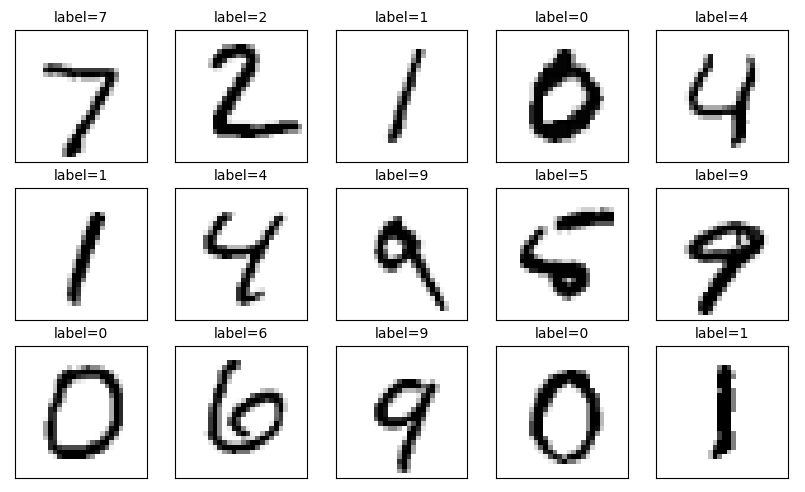
plot_images_labels_prediction(mnist.test.images,mnist.test.labels,prediction_result,0,15) #0代表下标从0幅开始,15表示最多显示15幅
运行结果为:

通过可视化,可以更直观的查看哪些预测对了 哪些预测错了。
plot_images_labels_prediction(mnist.test.images,mnist.test.labels,[],0,15)
如果参数预测列表设为空,也能执行,只不过不显示预测标签的值。这时函数相当于查看训练集,运行结果为:
完整代码如下


#Created by:Huang
#Time:2019/10/9 0009.
import tensorflow as tf
import tensorflow.examples.tutorials.mnist.input_data as input_data
import matplotlib.pyplot as plt
import numpy as np

mnist = input_data.read_data_sets("MNIST_data/",one_hot=True)
# print('训练集train 数量:',mnist.train.num_examples,',验证集 validation 数量:',mnist.validation.num_examples,',测试集test 数量:',mnist.test.num_examples)

# print('train images shape:',mnist.train.images.shape,'labels shaple:',mnist.train.labels.shape)
#(55000,784)意思是5w5千条,每一条784位(图片大小28*28);(55000,10):10分类 One Hot编码
# def plot_image(image):
#       plt.imshow(image.reshape(28,28),cmap='binary')
#       plt.show()
# plot_image(mnist.train.images[20000])
x = tf.placeholder(tf.float32,[None,784],name="X")#mnist 中每张图片共有28*28=784个像素点
y = tf.placeholder(tf.float32,[None,10],name="Y")#0-9一共10个数字=>10个类别

W= tf.Variable(tf.random_normal([784,10]),name="W")  #定义变量
b= tf.Variable(tf.zeros([10]),name="b")
#用单个神经元构建神经网络
forward = tf.matmul(x, W) + b  #前向计算
pred = tf.nn.softmax(forward)  #Softmax分类

train_epochs = 50   #训练轮数
batch_size=100      #单次训练样本数(批次大小)
total_batch= int(mnist.train.num_examples/batch_size)#一轮训练有多少批次
display_step=1     #显示粒度
learning_rate=0.01   #学习率

loss_function = tf.reduce_mean(-tf.reduce_sum(y*tf.log(pred),reduction_indices=1))   #定义交叉熵损失函数
optimizer = tf.train.GradientDescentOptimizer(learning_rate).minimize(loss_function)  #梯度下降优化器

#检查预测类别tf.argmax(pred,1)与实际类别tf.argmax(y.1)的匹配情况,argmax能把最大值的下标取出来
correct_prediction = tf.equal(tf.argmax(pred,1),tf.argmax(y,1))
#准确率,将布尔值转化为浮点数,并计算平均值
accuracy = tf.reduce_mean(tf.cast(correct_prediction,tf.float32))
sess = tf.Session()#声明会活
init = tf.global_variables_initializer()#变量初始化
sess.run(init)

#开始训练
for epoch in range(train_epochs):
    for batch in range(total_batch):
          xs,ys = mnist.train.next_batch(batch_size)  # 读取批次数据
          sess.run(optimizer,feed_dict={x:xs,y:ys})   # 执行批次训练
    #total_batch个批次训练完成后,使用验证数据计算课差与准确率;验证集没有分批
    loss,acc = sess.run([loss_function,accuracy],feed_dict={x:mnist.validation.images,y:mnist.validation.labels})
    #打印训练过程中的详细信息
    if (epoch+1) % display_step == 0:
        print("Train Epoch:",'%02d' %(epoch+1),"Loss=","{:.9f}".format(loss),"Accuracy=","{:.4f}".format(acc))
print("Train Finished!")


accu_test = sess.run(accuracy,feed_dict={x:mnist.test.images,y:mnist.test.labels})
print("Test Accuracy:",accu_test)

accu_train = sess.run(accuracy,feed_dict={x:mnist.train.images,y:mnist.train.labels})
print("Train Accuracy:",accu_train)

#模型预测
#由于pred预测结果是one-hot编码格式,所以需要转换为0-9数字
prediction_result = sess.run(tf.argmax(pred,1),feed_dict={x:mnist.test.images})

print(prediction_result[0:10])  #查看预测结果中的前10项


def plot_images_labels_prediction(images,labels,prediction,index,num=10):   #图像列表,标签列表,预测值列表,从第index个开始显示 , 缺省一次显示10幅
    fig = plt.gcf() #获取当前图表,get current figure
    fig.set_size_inches(10,12)  #1英寸等于2.54cm
    if num > 25:
        num = 25  #最多显示25个子图
    for i in range(0, num):
        ax = plt.subplot(5,5,i+1)  #获取当前要处理的子图
        ax.imshow(np.reshape(images[index], (28, 28)),cmap='binary')  # 显示第index个图像
        title = "label=" + str(np.argmax(labels[index]))# 构建该图上要显示的
        if len(prediction)>0:
            title += ",predict="+ str(prediction[index])
        ax.set_title(title, fontsize=10)  #显示图上title信息
        ax.set_xticks([])  #不显示坐标轴
        ax.set_yticks([])
        index += 1
    plt.show()


plot_images_labels_prediction(mnist.test.images,mnist.test.labels,prediction_result,0,15)  #最多显示25张
# plot_images_labels_prediction(mnist.test.images,mnist.test.labels,[],0,15)  #最多显示25张