一元回归:
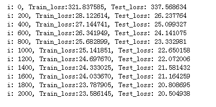
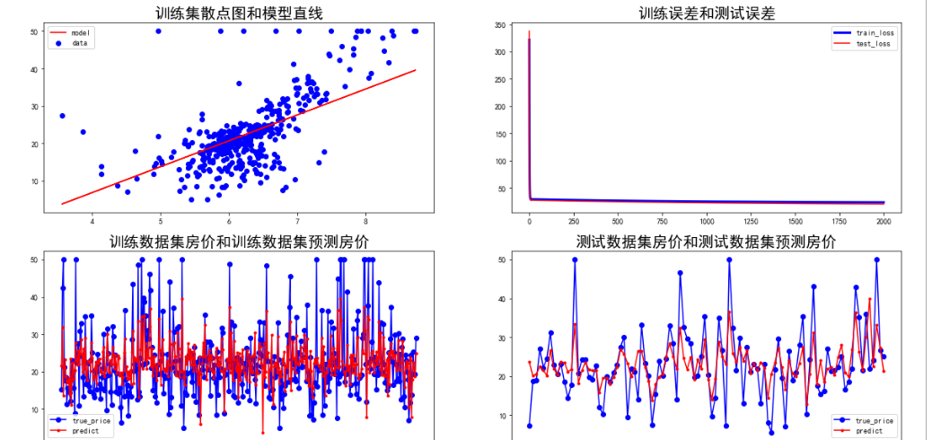
 1 import numpy as np
 2 import matplotlib.pyplot as plt
 3 import tensorflow as tf
 4
 5 #加载数据集
 6 boston_housing = tf.keras.datasets.boston_housing
 7 (train_x,train_y),(test_x,test_y) = boston_housing.load_data()
 8
 9 #数据处理
10 x_train= train_x[:,5]   #取出训练集房间这个属性
11 y_train = train_y      #为了和x_rain名字保持一致,重新命名
12
13 x_test = test_x[:,5]    #取出测试集中房间数学
14 y_test = test_y
15
16 #设置超参数
17 learn_rate = 0.04
18 iter = 2000
19 display_step=200
20
21 #设置模型参数初始值
22 np.random.seed(612)
23 w = tf.Variable(np.random.randn)
24 b = tf.Variable(np.random.randn)
25
26 #训练模型
27 mse_train = []   #记录训练误差
28 mse_test = []     #记录测试误差
29
30 for i in range(iter+1):
31     with tf.GradientTape() as tape:
32          #计算训练集的预测房价和误差
33         pred_train = w*x_train +b
34         loss_train = 0.5*tf.reduce_mean(tf.square(y_train-pred_train))
35
36         #计算测试集的预测房价和误差
37         pred_test = w*x_test +b
38         loss_test = 0.5*tf.reduce_mean(tf.square(y_test-pred_test))
39
40     mse_train.append(loss_train)
41     mse_test.append(loss_test)
42
43     dL_dw,dL_db = tape.gradient(loss_train, [w,b]) #第w和b进行求导
44     w.assign_sub(learn_rate*dL_dw)             #更新w和b
45     b.assign_sub(learn_rate*dL_db)
46
47     if i % display_step == 0:
48         print('i: %i, Train_loss:%f, Test_loss: %f' % (i,loss_train,loss_test))
49
50
51 #可视化输出
52 plt.figure(figsize=(20,10))
53
54 plt.subplot(221)
55 plt.scatter(x_train,y_train, color='blue', label = 'data')
56 plt.plot(x_train,pred_train, color = 'red', label='model')
57 plt.legend(loc='upper left')
58 plt.title('训练集散点图和模型直线',fontsize = 20)
59
60 plt.subplot(222)
61 plt.plot(mse_train, color='blue',linewidth=3, label='train_loss')
62 plt.plot(mse_test, color='red',linewidth=1.5, label='test_loss')
63 plt.legend(loc='upper right')
64 plt.title('训练误差和测试误差',fontsize = 20)
65
66 plt.subplot(223)
67 plt.plot(y_train,color='blue', marker='o', label='true_price')
68 plt.plot(pred_train, color ='red', marker='.', label='predict')
69 plt.legend()
70 plt.title('训练数据集房价和训练数据集预测房价',fontsize = 20)
71
72 plt.subplot(224)
73 plt.plot(y_test, color='blue', marker='o', label='true_price')
74 plt.plot(pred_test, color='red', marker='.', label='predict')
75 plt.legend()
76 plt.title('测试数据集房价和测试数据集预测房价',fontsize = 20)
77
78 plt.show()
多元回归:
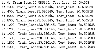
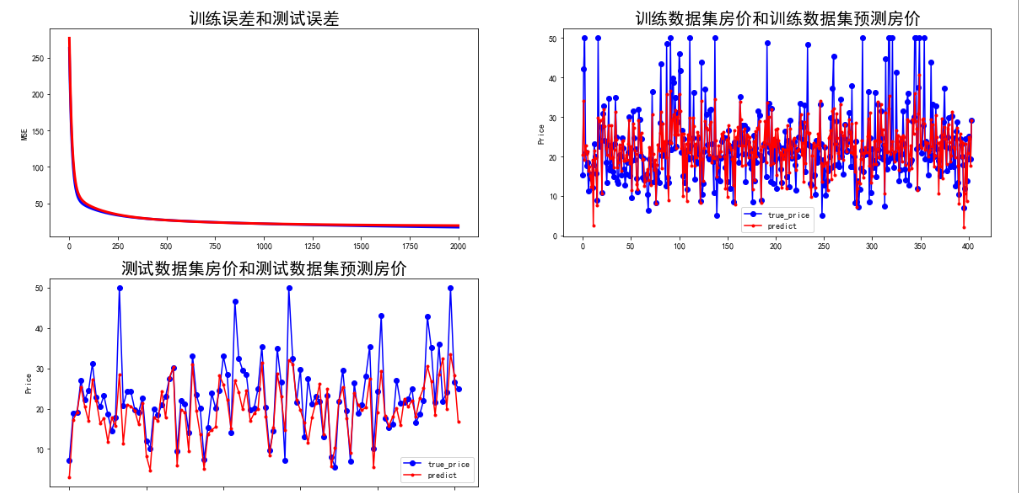
 1 import numpy as np
 2 import matplotlib.pyplot as plt
 3 import tensorflow as tf
 4
 5 #加载数据集
 6 boston_housing = tf.keras.datasets.boston_housing
 7 (train_x,train_y),(test_x,test_y) = boston_housing.load_data()
 8
 9 num_train=len(train_x)   #训练集和测试机中样本的数量
10 num_test=len(test_x)
11
12 #对训练样本和测试样本进行标准化(归一化),这里有用到张量的广播运算机制
13 x_train=(train_x-train_x.min(axis=0))/(train_x.max(axis=0)-train_x.min(axis=0))
14 y_train = train_y
15
16 x_test=(test_x-test_x.min(axis=0))/(test_x.max(axis=0)-test_x.min(axis=0))
17 y_test = test_y
18
19 #生成多元回归需要的二维形式
20 x0_train = np.ones(num_train).reshape(-1,1)
21 x0_test = np.ones(num_test).reshape(-1,1)
22
23     #对张量数据类型转换和进行堆叠
24 X_train = tf.cast(tf.concat([x0_train,x_train],axis=1), tf.float32)
25 X_test = tf.cast(tf.concat([x0_test, x_test], axis=1), tf.float32)
26
27 #将房价转换为列向量
28 Y_train = tf.constant(y_train.reshape(-1,1), tf.float32)
29 Y_test = tf.constant(y_test.reshape(-1,1), tf.float32)
30
31 #设置超参数
32 learn_rate = 0.01
33 iter = 2000
34 display_step=200
35
36 #设置模型变量初始值
37 np.random.seed(612)
38 W = tf.Variable(np.random.randn(14,1), dtype = tf.float32)
39
40 #训练模型
41 mse_train=[]
42 mse_test=[]
43
44 for i in range(iter+1):
45     with tf.GradientTape() as tape:
46         PRED_train = tf.matmul(X_train,W)
47         Loss_train = 0.5*tf.reduce_mean(tf.square(Y_train-PRED_train))
48
49         PRED_test = tf.matmul(X_test,W)
50         Loss_test = 0.5*tf.reduce_mean(tf.square(Y_test-PRED_test))
51
52     mse_train.append(Loss_train)
53     mse_test.append(Loss_test)
54
55     dL_dW = tape.gradient(Loss_train, W)
56     W.assign_sub(learn_rate*dL_dW)
57
58     if i % display_step == 0:
59         print('i: %i, Train_loss:%f, Test_loss: %f' % (i,loss_train,loss_test))
60
61
62 #可视化输出
63 plt.figure(figsize=(20,10))
64
65 plt.subplot(221)
66 plt.ylabel('MSE')
67 plt.plot(mse_train,color = 'blue',linewidth=3)
68 plt.plot(mse_test,color = 'red',linewidth=3)
69 plt.title('训练误差和测试误差',fontsize = 20)
70
71 plt.subplot(222)
72 plt.ylabel('Price')
73 plt.plot(y_train,color='blue', marker='o', label='true_price')
74 plt.plot(PRED_train, color ='red', marker='.', label='predict')
75 plt.legend()
76 plt.title('训练数据集房价和训练数据集预测房价',fontsize = 20)
77
78 plt.subplot(223)
79 plt.ylabel('Price')
80 plt.plot(y_test, color='blue', marker='o', label='true_price')
81 plt.plot(PRED_test, color='red', marker='.', label='predict')
82 plt.legend()
83 plt.title('测试数据集房价和测试数据集预测房价',fontsize = 20)
84
85 plt.show()