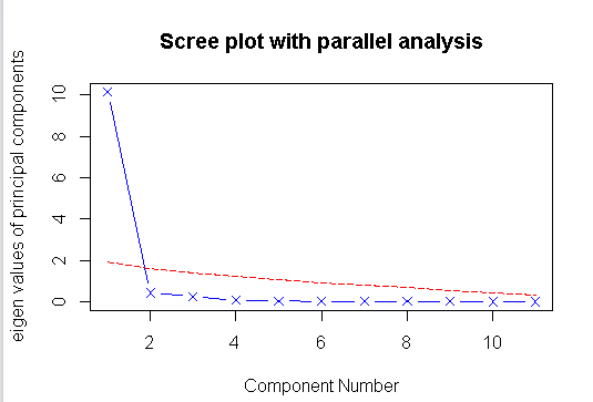
#主成分分析
par(mfrow=(c(1,1)))
library(psych)
head(USJudgeRatings,5)
head(USJudgeRatings[,-1],5)

fa.parallel(USJudgeRatings[,-1],fa="pc",n.iter=100,show.legend = FALSE,main="Scree plot with parallel analysis")
#如下图,发现测试的数据中,有一个主要成分
#提取主成分
pc<-principal(USJudgeRatings[,-1],nfactors=1)
pc
Principal Components Analysis
Call: principal(r = USJudgeRatings[, -1], nfactors = 1)
Standardized loadings (pattern matrix) based upon correlation matrix
PC1 h2 u2 com
INTG 0.92 0.84 0.1565 1
DMNR 0.91 0.83 0.1663 1
DILG 0.97 0.94 0.0613 1
CFMG 0.96 0.93 0.0720 1
DECI 0.96 0.92 0.0763 1
PREP 0.98 0.97 0.0299 1
FAMI 0.98 0.95 0.0469 1
ORAL 1.00 0.99 0.0091 1
WRIT 0.99 0.98 0.0196 1
PHYS 0.89 0.80 0.2013 1
RTEN 0.99 0.97 0.0275 1
PC1
SS loadings 10.13
Proportion Var 0.92
Mean item complexity = 1
Test of the hypothesis that 1 component is sufficient.
The root mean square of the residuals (RMSR) is 0.04
with the empirical chi square 6.2 with prob < 1
Fit based upon off diagonal values = 1
#例子,身体测量指标主成份分析
library(psych)
fa.parallel(Harman23.cor$cov,n.obs=302,fa="pc",n.iter=100,show.legend = FALSE,main="Scree plot with parallel analysis")

pc<-principal(Harman23.cor$cov,nfactors=2,rotate="none")
pc
Principal Components Analysis
Call: principal(r = Harman23.cor$cov, nfactors = 2, rotate = "none")
Standardized loadings (pattern matrix) based upon correlation matrix
PC1 PC2 h2 u2 com
height 0.86 -0.37 0.88 0.123 1.4
arm.span 0.84 -0.44 0.90 0.097 1.5
forearm 0.81 -0.46 0.87 0.128 1.6
lower.leg 0.84 -0.40 0.86 0.139 1.4
weight 0.76 0.52 0.85 0.150 1.8
bitro.diameter 0.67 0.53 0.74 0.261 1.9
chest.girth 0.62 0.58 0.72 0.283 2.0
chest.width 0.67 0.42 0.62 0.375 1.7
PC1 PC2
SS loadings 4.67 1.77
Proportion Var 0.58 0.22
Cumulative Var 0.58 0.81
Proportion Explained 0.73 0.27
Cumulative Proportion 0.73 1.00
Mean item complexity = 1.7
Test of the hypothesis that 2 components are sufficient.
The root mean square of the residuals (RMSR) is 0.05
Fit based upon off diagonal values = 0.99
#主成份旋转
rc<-principal(Harman23.cor$cov,nfactors = 2,rotate="varimax")
rc
Principal Components Analysis
Call: principal(r = Harman23.cor$cov, nfactors = 2, rotate = "varimax")
Standardized loadings (pattern matrix) based upon correlation matrix
RC1 RC2 h2 u2 com
height 0.90 0.25 0.88 0.123 1.2
arm.span 0.93 0.19 0.90 0.097 1.1
forearm 0.92 0.16 0.87 0.128 1.1
lower.leg 0.90 0.22 0.86 0.139 1.1
weight 0.26 0.88 0.85 0.150 1.2
bitro.diameter 0.19 0.84 0.74 0.261 1.1
chest.girth 0.11 0.84 0.72 0.283 1.0
chest.width 0.26 0.75 0.62 0.375 1.2
RC1 RC2
SS loadings 3.52 2.92
Proportion Var 0.44 0.37
Cumulative Var 0.44 0.81
Proportion Explained 0.55 0.45
Cumulative Proportion 0.55 1.00
Mean item complexity = 1.1
Test of the hypothesis that 2 components are sufficient.
The root mean square of the residuals (RMSR) is 0.05
Fit based upon off diagonal values = 0.99
#获取每个变量在主成份上的得分
pc<-principal(USJudgeRatings[,-1],nfactors=1,score=TRUE)
head(pc$scores)
PC1
AARONSON,L.H. -0.19
ALEXANDER,J.M. 0.75
ARMENTANO,A.J. 0.07
BERDON,R.I. 1.14
BRACKEN,J.J. -2.16
BURNS,E.B. 0.77
#获取主成分得分系数
rc<-principal(Harman23.cor$cov,nfactors=2,rotate="varimax")
round(unclass(rc$weights),2)
RC1 RC2
height 0.28 -0.05
arm.span 0.30 -0.08
forearm 0.30 -0.09
lower.leg 0.28 -0.06
weight -0.06 0.33
bitro.diameter -0.08 0.32
chest.girth -0.10 0.34
chest.width -0.04 0.27
#探索性因子分析
#整理测试数据
options(digits=2)
covariances<-ability.cov$cov
correlations<-cov2cor(covariances)
correlations
general picture blocks maze reading vocab
general 1.00 0.47 0.55 0.34 0.58 0.51
picture 0.47 1.00 0.57 0.19 0.26 0.24
blocks 0.55 0.57 1.00 0.45 0.35 0.36
maze 0.34 0.19 0.45 1.00 0.18 0.22
reading 0.58 0.26 0.35 0.18 1.00 0.79
vocab 0.51 0.24 0.36 0.22 0.79 1.00
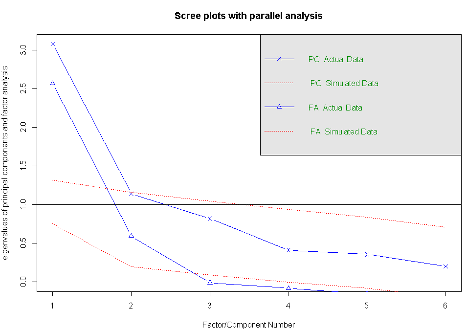
#判断需提取的公共因子数,本例中显示的结果为:有两个因子可以获取
fa.parallel(correlations,n.obs=112,fa="both",n.iter=100,main="Scree plots with parallel analysis")
#提取公共因子
fa<-fa(correlations,nfactors=2,rotate="none",fm="pa")  #nfactors指出需要提取的因子数
fa
Factor Analysis using method = pa
Call: fa(r = correlations, nfactors = 2, rotate = "none", fm = "pa")
Standardized loadings (pattern matrix) based upon correlation matrix
PA1 PA2 h2 u2 com
general 0.75 0.07 0.57 0.432 1.0
picture 0.52 0.32 0.38 0.623 1.7
blocks 0.75 0.52 0.83 0.166 1.8
maze 0.39 0.22 0.20 0.798 1.6
reading 0.81 -0.51 0.91 0.089 1.7
vocab 0.73 -0.39 0.69 0.313 1.5
PA1 PA2
SS loadings 2.75 0.83
Proportion Var 0.46 0.14
Cumulative Var 0.46 0.60
Proportion Explained 0.77 0.23
Cumulative Proportion 0.77 1.00
Mean item complexity = 1.5
Test of the hypothesis that 2 factors are sufficient.
The degrees of freedom for the null model are 15 and the objective function was 2.5
The degrees of freedom for the model are 4 and the objective function was 0.07
The root mean square of the residuals (RMSR) is 0.03
The df corrected root mean square of the residuals is 0.06
Fit based upon off diagonal values = 0.99
Measures of factor score adequacy
PA1 PA2
Correlation of scores with factors 0.96 0.92
Multiple R square of scores with factors 0.93 0.84
Minimum correlation of possible factor scores 0.86 0.68
#因子旋转
#正交旋转
fa.varimax<-fa(correlations,nfactors=2,rotate="varimax",fm="pa")
fa.varimax
Factor Analysis using method = pa
Call: fa(r = correlations, nfactors = 2, rotate = "varimax", fm = "pa")
Standardized loadings (pattern matrix) based upon correlation matrix
PA1 PA2 h2 u2 com
general 0.49 0.57 0.57 0.432 2.0
picture 0.16 0.59 0.38 0.623 1.1
blocks 0.18 0.89 0.83 0.166 1.1
maze 0.13 0.43 0.20 0.798 1.2
reading 0.93 0.20 0.91 0.089 1.1
vocab 0.80 0.23 0.69 0.313 1.2
PA1 PA2
SS loadings 1.83 1.75
Proportion Var 0.30 0.29
Cumulative Var 0.30 0.60
Proportion Explained 0.51 0.49
Cumulative Proportion 0.51 1.00
Mean item complexity = 1.3
Test of the hypothesis that 2 factors are sufficient.
The degrees of freedom for the null model are 15 and the objective function was 2.5
The degrees of freedom for the model are 4 and the objective function was 0.07
The root mean square of the residuals (RMSR) is 0.03
The df corrected root mean square of the residuals is 0.06
Fit based upon off diagonal values = 0.99
Measures of factor score adequacy
PA1 PA2
Correlation of scores with factors 0.96 0.92
Multiple R square of scores with factors 0.91 0.85
Minimum correlation of possible factor scores 0.82 0.71
#斜交旋转
install.packages("GPArotation")
library(GPArotation)
fa.promax<-fa(correlations,nfactors=2,rotate="promax",fm="pa")
fa.promax
Factor Analysis using method = pa
Call: fa(r = correlations, nfactors = 2, rotate = "promax", fm = "pa")
Warning: A Heywood case was detected.
Standardized loadings (pattern matrix) based upon correlation matrix
PA1 PA2 h2 u2 com
general 0.37 0.48 0.57 0.432 1.9
picture -0.03 0.63 0.38 0.623 1.0
blocks -0.10 0.97 0.83 0.166 1.0
maze 0.00 0.45 0.20 0.798 1.0
reading 1.00 -0.09 0.91 0.089 1.0
vocab 0.84 -0.01 0.69 0.313 1.0
PA1 PA2
SS loadings 1.83 1.75
Proportion Var 0.30 0.29
Cumulative Var 0.30 0.60
Proportion Explained 0.51 0.49
Cumulative Proportion 0.51 1.00
With factor correlations of
PA1 PA2
PA1 1.00 0.55
PA2 0.55 1.00
Mean item complexity = 1.2
Test of the hypothesis that 2 factors are sufficient.
The degrees of freedom for the null model are 15 and the objective function was 2.5
The degrees of freedom for the model are 4 and the objective function was 0.07
The root mean square of the residuals (RMSR) is 0.03
The df corrected root mean square of the residuals is 0.06
Fit based upon off diagonal values = 0.99
Measures of factor score adequacy
PA1 PA2
Correlation of scores with factors 0.97 0.94
Multiple R square of scores with factors 0.93 0.88
Minimum correlation of possible factor scores 0.86 0.77
#显示因子的相关系数?
fsm<-function(oblique){
if(class(oblique)[2] =="fa" & is.null(oblique$Phi)){
warning("Object dosen't look like oblique EFA")
} else{
P<-unclass(oblique$loading)
F<-P%*% oblique$Phi
colnames(F)<-c("PA1","PA2")
return(F)
}
}
fsm(fa.promax)
PA1 PA2
general 0.64 0.69
picture 0.32 0.61
blocks 0.43 0.91
maze 0.25 0.45
reading 0.95 0.46
vocab 0.83 0.45
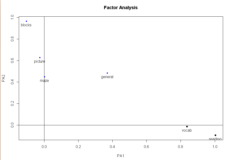
#斜交结果的图形展示
factor.plot(fa.promax,labels=rownames(fa.promax$loadings))
#因子关联图
fa.diagram(fa.promax,simple=FALSE)

#因子得分
fa.promax$weights
PA1 PA2
general 0.078 0.211
picture 0.020 0.090
blocks 0.037 0.702
maze 0.027 0.035
reading 0.743 0.030
vocab 0.177 0.036
总的来说,成分分析和公因子分析都是用来探索哪些因子是用来构建模型的最优选择。