线性回归(Linear Regression)
理论实现
最简单的想法是
[y approx sum _ { i = 0 } ^ { d } w _ { i } x _ { i }
]
线性回归的假设函数为: (h(mathrm{x}) = mathrm{w}^{T} mathrm{x})。类似于 perceptron 只是没有 sign 函数。
线性回归的目的是找到一个方差最小的超平面(线条),所以误差检测使用流行的方差(squared error)
[operatorname{err}( ilde{y}, y) =( ilde{y}-y)^{2}
]
in-sample / out-of-sample 误差为:
[E _ { mathrm { in } } ( mathbf { w } ) = frac { 1 } { N } sum _ { n = 1 } ^ { N } ( underbrace { h left( mathbf { x } _ { n }
ight) } _ { mathbf { w } ^ { T } mathbf { x } _ { n } } - y _ { n } ) ^ { 2 }\
E _ { ext {out } } ( mathbf { w } ) = underset { ( mathbf { x } , y ) sim P } { mathcal { E } } left( mathbf { w } ^ { T } mathbf { x } - y
ight) ^ { 2 }
]
为了表示方便写出 in-sample 误差 (E _ { mathrm { in } } ( mathbf { w } )) 的矩阵形式:
[�egin{aligned} E _ { mathrm { in } } ( mathbf { w } )
& = frac { 1 } { N } sum _ { n = 1 } ^ { N } left( mathbf { w } ^ { T } mathbf { x } _ { n } - y _ { n }
ight) ^ { 2 } = frac { 1 } { N } sum _ { n = 1 } ^ { N } left( mathbf { x } _ { n } ^ { T } mathbf { w } - y _ { n }
ight) ^ { 2 } \
&= frac { 1 } { N } left| �egin{array} { c } mathbf { x } _ { 1 } ^ { T } mathbf { w } - y _ { 1 } \ mathbf { x } _ { 2 } ^ { T } mathbf { w } - y _ { 2 } \ cdots \ mathbf { x } _ { N } ^ { T } mathbf { w } - y _ { N } end{array}
ight| ^ { 2 }\
&= frac { 1 } { N } left| left[ �egin{array} { c } - - mathbf { x } _ { 1 } ^ { T } - - \ - - mathbf { x } _ { 2 } ^ { T } - - \ cdots \ - - mathbf { x } _ { N } ^ { T } - - end{array}
ight] mathbf { w } - left[ �egin{array} { c } y _ { 1 } \ y _ { 2 } \ cdots \ y _ { N } end{array}
ight]
ight| ^ { 2 }\
& = frac { 1 } { N } | underbrace { X } _ { N imes d + 1 } underbrace { mathbf { w } } _ { d + 1 imes 1 } - underbrace { mathbf { y } } _ { N imes 1 } | ^ { 2 }
end{aligned}
]
那现在的任务便是
[min _ { w } E _ { i n } ( mathbf { w } ) = frac { 1 } { N } | X mathbf { w } - mathbf { y } | ^ { 2 }
]
此时的 (E _ { mathrm { in } } ( mathbf { w } )) 曲线如下:
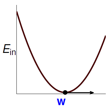
由公式和图形可知 (E _ { mathrm { in } } ( mathbf { w } )) 是连续(continuous),可微(differentiable),凸(convex)的。那么最小化 (E _ { mathrm { in } } ( mathbf { w } )) 的必要条件(necessary condition)是:
[
abla E _ { ext {in } } ( mathbf { w } ) equiv left[ �egin{array} { c } frac { partial E _ { ext {in } } } { partial w _ { 0 } } ( mathbf { w } ) \ frac { partial E _ { ext {in } } } { partial w _ { 1 } } ( mathbf { w } ) \ cdots \ frac { partial E _ { ext {in } } } { partial w _ { d } } ( mathbf { w } ) end{array}
ight] = left[ �egin{array} { c } 0\ 0\ cdots\ 0\ end{array}
ight]
]
那么现在的任务便是找出(mathbf{w}_{LIN}) 使得 (
abla E _ { ext {in } }(mathbf{w}_{LIN}) = 0)。
矩阵形式的多项式展开为:
[E _ { mathrm { in } } ( mathbf { w } ) = frac { 1 } { N } | mathrm { Xw } - mathbf { y } | ^ { 2 } = frac { 1 } { N } left( mathbf { w } ^ { T } mathbf { X } ^ { T } mathbf { X } mathbf { w } - 2 mathbf { w } ^ { T } mathbf { X } ^ { T } mathbf { y } + mathbf { y } ^ { T } mathbf { y }
ight)
]
所以其矩阵求导结果为(可类比于非向量形式):
[
abla E _ { ext {in } } ( mathbf { w } ) = frac { 2 } { N } left( X ^ { T } X mathbf { w } - X ^ { T } mathbf { y }
ight)
]
那么现在令其为零可求得:
[mathbf { w } _ { mathrm { LIN } } = mathrm { X } ^ { dagger } mathbf { y }
]
其中 ({ dagger }) 代表伪逆,当(mathrm { X }^{T} mathrm { X })非奇异时也可使用 (mathbf { w } _ { mathrm { LIN } } = (mathrm { X }^{T} mathrm { X })^{-1} mathrm { X } mathbf { y }) 求得。
总结一下Linear Regression算法的实现步骤为:
- 通过数据集,获取输入矩阵(input matrix)和输出向量(output vector)
[X = underbrace{left[ �egin{array} { c } - - mathbf { x } _ { 1 } ^ { T } - - \ - - mathbf { x } _ { 2 } ^ { T } - - \ cdots \ - - mathbf { x } _ { N } ^ { T } - - end{array}
ight]}_{N imes (d+1)} \,\,\,\,\,\,\,\,\,\, mathbf{y} = underbrace{left[ �egin{array} { c } y _ { 1 } \ y _ { 2 } \ cdots \ y _ { N } end{array}
ight]}_{N imes 1} \
]
- 计算伪逆 (pseudo-inverse)(underbrace{mathrm { X } ^ { dagger }}_{(d+1) imes N})
- return (underbrace{mathbf { w } _ { mathrm { LIN } }}_{d+1 imes 1} = mathrm { X } ^ { dagger } mathbf { y })
Hat Matrix 的几何视角
下面公式的意义为对于服从统一分布的数据,经过多次抽取后训练误差的平均 (overline{E _ { ext {in } }}),而其大概长下面这个样子是
[overline{E _ { ext {in } }} = underset { mathcal { D } _ { sim P N } } { mathcal { E } } left{ E _ { ext {in } } left( mathbf { w } _ { ext {LIN } } ext { w.r.t. } mathcal { D }
ight)
ight} = ext{noise level} cdot left( 1 - frac { d + 1 } { N }
ight)
]
[�egin{aligned}
E _ { mathrm { in } } left( mathbf { w } _ { mathrm { LIN } }
ight) = frac { 1 } { N } | mathbf { y } - underbrace { hat { mathbf { y } } } _ { ext {predictions } } | ^ { 2 }
& = frac { 1 } { N } | mathbf { y } - mathrm { X } underbrace { mathrm { X } ^ { dagger } mathbf { y } } _ { mathrm { W } _ { mathrm { LIN } } } | ^ { 2 }\
& = frac { 1 } { N } | (underbrace{mathbf { I }}_{ ext{identity}} - mathrm { X } underbrace { mathrm { X } ^ { dagger }) mathbf { y } } _ { mathrm { W } _ { mathrm { LIN } } } | ^ { 2 }
end{aligned}
]
这里叫 (mathrm { X } mathrm { X } ^ {dagger}) 为 hat matrix (H)。
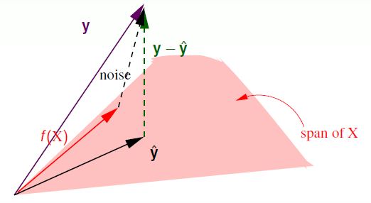
经过上述推导,可以得出 (hat {mathbf { y } }= mathrm { X }mathbf { w } _ { mathrm { LIN } }) ,即 (hat {mathbf { y } }) 是 (mathbf{x}_{n}) 的线性组合,也是由 (mathbf{x}_{n}) 展开的空间中的一个向量;同时由于 (mathbf { y }) 是独立于该空间外的一个向量,同时由于 (mathbf { y }-hat {mathbf { y } }) 最小,那么 (mathbf { y }-hat {mathbf { y } }) 必然垂直于该空间。进而可以得出 (hat {mathbf { y } }) 是 (mathbf { y }) 在该空间上的一个投影,而投影矩阵便是 (H)。所以 (I - H) 也可以看作 (mathbf { y }) 向 (mathbf { y }-hat {mathbf { y } }) 映射的投影矩阵。
可以推导得 ( ext{trace}(I - H) = N - (d + 1)),不详细解释。物理意义是将一个(N)维向量向(d+1)维空间做投影时,其余数的自由度最多有只有(N - (d + 1))。
那么 noise 向量向该空间内投影后取余仍然是 (( mathbf { I } - mathrm { H } ) ext{noise} = mathbf { y }-hat {mathbf { y } }) ,即:
[�egin{aligned} E _ { ext {in } } left( mathbf { w } _ { mathrm { LIN } }
ight) = frac { 1 } { N } | mathbf { y } - hat { mathbf { y } } | ^ { 2 } & = frac { 1 } { N } | ( mathbf { I } - mathrm { H } ) ext { noise } | ^ { 2 } \
& = frac { 1 } { N } ( N - ( d + 1 ) ) {| ext{noise} |} ^ { 2 } \
& = frac { 1 } { N } ( N - ( d + 1 ) ) sigma ^ { 2 }
end{aligned}
]
经过理论推导可以得出(这里不详细推导):
[�egin{aligned}
overline{E _ { ext {in} }} &= ( 1 - frac { d + 1 } { N } ) sigma ^ { 2 } \
overline{E _ { ext {out} }} &= ( 1 + frac { d + 1 } { N } ) sigma ^ { 2 }
end{aligned}
]
将两者绘制出随数据量增加的变化曲线如下:
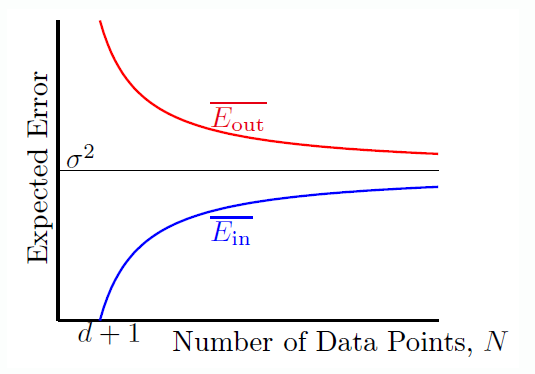
可以看出当 (N
ightarrow inf) 时,两者均收敛,且两者之差为 (frac { 2(d + 1) } { N })。类似于 VC bound。
线性回归(Linear Regression)(
ightarrow)分类(Classification)
由于 Linear Classification 是一种 NP-Hard 问题,那可以将回归的解决方法用于分类吗?
先对比一下两者的误差测量函数:
[operatorname { err } _ { 0 / 1 } = left| operatorname { sign } left( mathbf { w } ^ { T } mathbf { x }
ight)
eq y
ight| quad ext { err } _ { mathrm { sqr } } = left( mathbf { w } ^ { T } mathbf { x } - y
ight) ^ { 2 }
]
绘制出曲线如下:
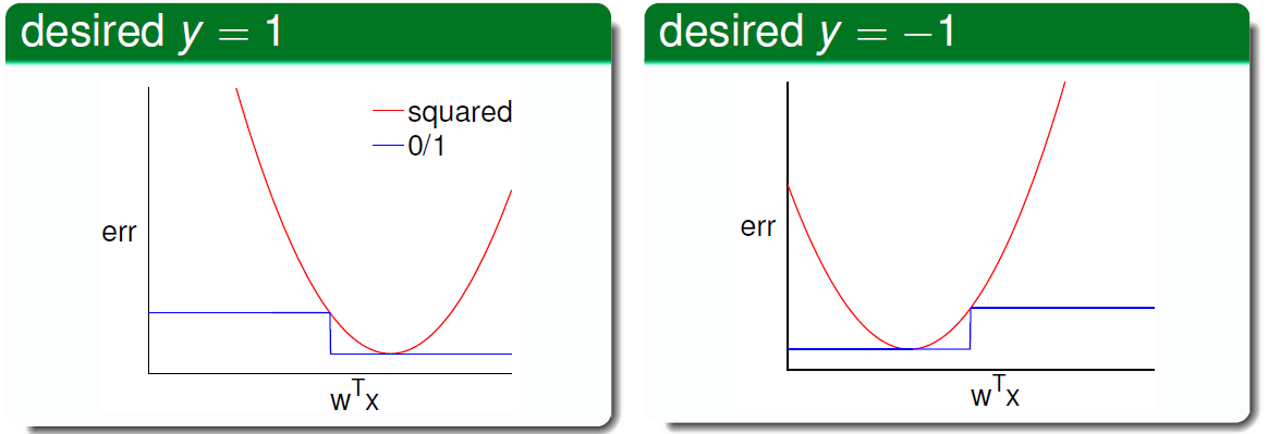
可见(operatorname { err } _ { 0 / 1 } < operatorname { err } _ { ext{sqr} }),所以可以得出:
[�egin{aligned}
ext{classification } E_{out}(mathbf{w})
& leq ext{classification } E_{in}(mathbf{w}) + sqrt{cdots cdots} \
& leq ext{regression } E_{in}(mathbf{w}) + sqrt{cdots cdots}
end{aligned}
]
所以说如果回归误差作为上限很小,那么分类误差也会很小。所以线性回归可以用于分类。
由于存在误差所以可以将(mathbf{w}_{LIN})作为 PLA/Pocket 算法的初始(基础)向量。