[�egin{array} { c | | c | c } ext { aggregation type } & ext { blending } & ext { learning } \ hline hline ext { uniform } & ext { voting/averaging } & ext { Bagging } \ hline ext { non-uniform } & ext { linear } & ext { AdaBoost } \ hline ext { conditional } & ext { stacking } & ext { Decision Tree } end{array}
]
在前文介绍过 blending ,这实际上就是 meta algorithm,只是将已获得的假设函数做一个融合。
而 bagging 属于 learing 的一种,也就是说在融合过程中获取假设函数。bagging 与 AdaBoost 区别于一个是 uniform 而另一个不是。而 stacking 实际上就是将已有的假设函数集的输出作为特征输入到一个机器学习模型中,在训练出一个融合模型,当然可以是 PLA 等算法。决策树与stacking不同的地方在于,不需要预先训练处 (g_t),而是在学习过程中获得。
下面以为是否观看视频做决策的决策树示意图如下:
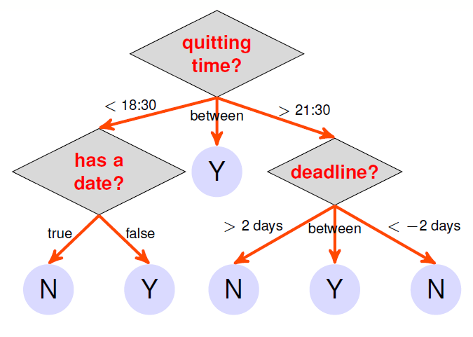
那么该决策树的数学表达如下:
[G ( mathbf { x } ) = sum _ { t = 1 } ^ { T } q _ { t } ( mathbf { x } ) cdot g _ { t } ( mathbf { x } )
]
其中 (g_t(mathbf{x})) 也是一个决策树,(q_t(mathbf{x})) 表示的是 (mathbf{x}) 是否在 (G) 的路径 (t) 中。由此看来决策树是一种仿人模型(human-mimicking models)。
从递推(树)的角度看:
[G ( mathbf { x } ) = sum _ { c = 1 } ^ { C } left[ kern-0.15em left[ b ( mathbf { x } ) = c
ight]kern-0.15em
ight]cdot G _ { c } ( mathbf { x } )
]
其中
- (G(x)) : full-tree hypothesis(当前根节点的全树模型)
- (b(x)) : branching criteria(判断是哪个分支)
- (G_c(x)): sub-tree hypothesis at the c-th branch(第c个分支的子树)
那么决策树的训练过程为:
[�egin{array} { l } ext { function Decision Tree } left( ext { data } mathcal { D } = left{ left( mathbf { x } _ { n } , y _ { n }
ight)
ight} _ { n = 1 } ^ { N }
ight) \ ext { if termination criteria met } \ ext { return base hypothesis } g _ { t } ( mathbf { x } ) \ ext { else } \ qquad �egin{array} { l } ext { learn branching criteria } b ( mathbf { x } ) \ ext { split } mathcal { D } ext { to } ext {C parts } mathcal { D } _ { c } = left{ left( mathbf { x } _ { n } , y _ { n }
ight) : b left( mathbf { x } _ { n }
ight) = c
ight} \ ext { build sub-tree } G _ { c } leftarrow ext { Decision Tree } left( mathcal { D } _ { c }
ight) \ ext { return } G ( mathbf { x } ) = sum _ { c = 1 } ^ { C } left[ kern-0.15em left[ b ( mathbf { x } ) = c
ight]kern-0.15em
ight]cdot G _ { c } ( mathbf { x } ) end{array} end{array}
]
从直观训练过程中,可以得知现在需要确认四个问题:
- number of branches(分支个数)(C)
- branching criteria(分支条件)(b ( mathbf { x } ))
- termination criteria(终止条件)
- base hypothesis(基假设函数)(g_t( mathbf { x } ))
由于有这么多可选条件,那么决策树模型有很多种实现方法,所以决策树模型有很多前人的巧思但是很有用(decision tree: mostly heuristic but useful on its own)。
下面介绍一个常用的决策树模型 —— Classification and Regression Tree(C&RT)
C&RT 模型
四个选择
其在前文所提到的四个问题的是如何解决的呢:
- 分支个数为 2 (二叉树),使用 decision stump (即 (b( mathbf { x })) 的实现方法)进行分段。
- 分支条件 (b( mathbf { x })) 也就是如何分支,最佳分支函数(模型)的选取,使用的是两部分数据是否 “纯” ,首先判断每段数据的纯度然后求平均值,作为本 decision stump 是否被选取的评价标准。
[b ( mathbf { x } ) = underset { ext { decision stumps } h ( mathbf { x } ) } { operatorname { argmin } } sum _ { c = 1 } ^ { 2 } | mathcal { D } _ { c } ext { with } h | cdot ext { impurity } left( mathcal { D } _ { c } ext { with } h
ight)
]
- 基假设函数 (g_t) 则是常值。
- 终止条件则是不能在分支(全部的 (y_n) 或 (mathbf{x}_n) 都一样,也就是说不纯度为零或者无法再进行决策时停止)。
详细实现
C&RT 模型 的 具体实现:
[�egin{array} { l }
ext { function Decision Tree } left( ext { data } mathcal { D } = left{ left( mathbf { x } _ { n } , y _ { n }
ight)
ight} _ { n = 1 } ^ { N }
ight) \ ext { if cannot branch anymore } \ qquad ext { return } g _ { t } ( mathbf { x } ) = E _ { ext {in } } ext { -optimal constant } \
ext { else learn branching criteria } \
qquad �egin{aligned}
& b ( mathbf { x } ) = operatorname { argmin } sum _ { ext {decision stumps } h ( mathbf { x } ) } sum _ { c = 1 } ^ { 2 } | mathcal { D } _ { c } ext { with } h | cdot ext { impurity } left( mathcal { D } _ { c } ext { with } h
ight) \
& ext { split } mathcal { D } ext { to } 2 ext { parts } mathcal { D } _ { c } = left{ left( mathbf { x } _ { n } , y _ { n }
ight) : b left( mathbf { x } _ { n }
ight) = c
ight} \
& ext { build sub-tree } G _ { c } leftarrow ext { Decision Tree } left( mathcal { D } _ { c }
ight) \
& ext { return } G ( mathbf { x } ) = sum _ { c = 1 } ^ { C } left[ kern-0.15em left[ b ( mathbf { x } ) = c
ight]kern-0.15em
ight]cdot G _ { c } ( mathbf { x } )
end{aligned}
end{array}
]
该决策树模型可以轻松驾驭回归,二分类和多分类。
不纯度函数(Impurity Functions)
回归错误(regression error)
用于回归,且是比较常用的方法
[�egin{array} { l } ext { impurity } ( mathcal { D } ) = frac { 1 } { N } sum _ { n = 1 } ^ { N } left( y _ { n } - �ar { y }
ight) ^ { 2 } \ ext { with } �ar { y } = ext { average of } left{ y _ { n }
ight} end{array}
]
将平均值作为评判标准。
分类错误(classification error)
用于分类
[�egin{array} { l } ext { impurity } ( mathcal { D } ) = frac { 1 } { N } sum _ { n = 1 } ^ { N } left[ y _ { n }
eq y ^ { * }
ight] \ ext { with } y ^ { * } = ext { majority of } left{ y _ { n }
ight} end{array}
]
将占比最多的类作为评判标准。
基尼系数(Gini index)
用于分类,且是比较常用的方法
[1 - sum _ { k = 1 } ^ { K } left( frac { sum _ { n = 1 } ^ { N } left[ kern-0.15em left[ { y } _ { n } = k
ight] kern-0.15em
ight] } { N }
ight) ^ { 2 }
]
考虑全部的类,计算不纯度。
剪枝正则化(Regularization by Pruning)
当全部的 (mathbf{x}_n) 均不相同,那么 (E_{in}(G) = 0),也就是说这是一个完全长成的树,这样会导致过拟合,因为在低位的子树构建数据很少,所以很容导致过拟合。所以这里想到使用剪枝实现正则化,简单来说就是控制数的叶子数量。
将叶子数量用 (Omega ( G )) 表示:
[Omega ( G ) = ext { NumberOfLeaves } ( G )
]
那么正则化后的优化目标则变为:
[underset { ext { all possible } G } { operatorname { argmin } } E _ { ext {in } } ( G ) + lambda Omega ( G )
]
做此操作后被叫做 被砍过的决策树(pruned decision tree)。
这里有一个比较困难的问题,那就是 ( ext { all possible } G),全部穷举是不可能的,在 C&RT 中,采用了以下策略:
[�egin{array} { l } G ^ { ( 0 ) } = ext { fully-grown tree } \ G ^ { ( i ) } = operatorname { argmin } _ { G } E _ { ext {in } } ( G ) ext { such that } G ext { is one-leaf removed from } G ^ { ( i - 1 ) } end{array}
]
也就是说在 摘掉 (i) 片树叶的决策树中找出性能最优的一颗,该决策树由摘掉 (i -1) 片树叶的决策树中最优的一颗再摘掉一片获得。
那么假设完全长成的决策树的叶子数量为 (I),那么现在便可以获得:
[G ^ { ( 0 ) },G ^ { ( 1 ) },cdots,G ^ { ( I^- ) } quad ext{where } I^{-} leq I
]
那么在从这一堆 (G^{(i)}) 中使用正则化的优化目标找出最优的那颗决策树。当然这里还有一个参数 (lambda) ,其可以用 validation 获得。
分类特征(Categorical Features)
在连续特征中,分支条件实现如下:
[�egin{aligned} & b ( mathbf { x } ) = left[ kern-0.15em left[ x _ { i } leq heta
ight] kern-0.15em
ight] + 1 \
ext{with } & heta in R
end{aligned}
]
而在离散特征中,分支条件类似
[�egin{aligned} & b ( mathbf { x } ) = left[ kern-0.15em left[ x _ { i } in S
ight] kern-0.15em
ight] + 1 \ ext{with }& S subset { 1,2 , ldots , K } end{aligned}
]
所以说决策树也很容易处理离散特征,或者说分类特征。
特征值缺失(Missing Features)
当你在做决策时,遇到特征值缺失你会怎么办呢,假如说这个特征是体重,我估计你会从身高和三维出发,估计这个人的大概的体重,因为你在决策过程中只是跟一个固定值做比较而已,所以不用太精准。
具体怎么做呢?数学表达如下:
[ ext { threshold on height } approx ext { threshold on weight }
]
也就是说体重缺失的话那就按身高划分
那么在 C&RT 中是找出并存储替代分支应对预测过程中的特征值缺失问题:
[ ext { surrogate branch } b _ { 1 } ( mathbf { x } ) , b _ { 2 } ( mathbf { x } ) , ldots approx ext { best branch } b ( mathbf { x } )
]
所以 C&RT 也很容易处理特征缺失问题。
举例说明(a simple dataset)
简单的举例说明
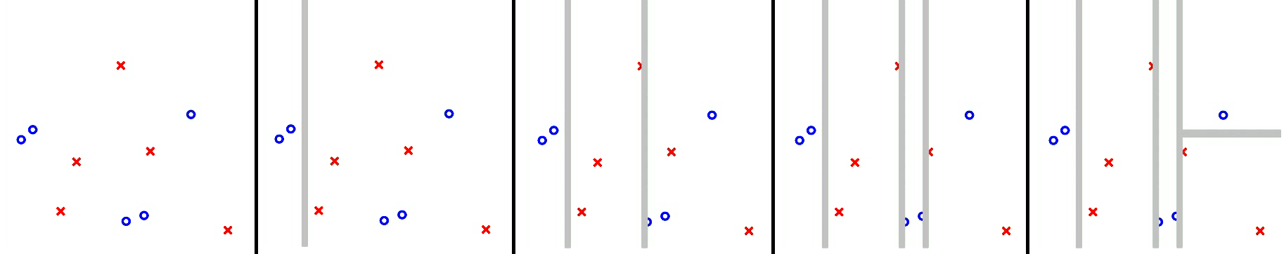
从左向右是决策树的学习过程,实际上就是不断的在不纯的区域进行划分,直到不纯度为零。
以此可以看出 AdaBoost-Stump 是在全局数据上进行分割,而 decision tree 则是在条件上在进行分割,如果不理解可以点击博文 机器学习技法 之 聚合模型(Aggregation Model) 观察AdaBoost-Stump 的学习过程。
值得注意的是另一个常用的决策树算法是 C4.5,区别是巧思不同(different choices of heuristics)。