使用Python的seaborn画热力图heatmap以及将两个矩阵合并画热图的方法

需要画一个这样的热图：

heatmap:

下面介绍具体过程：

　　1.原始数据为两个矩阵：rmsd_array,tm_rmsd_array

<class 'numpy.ndarray'>

array([[ 0.   , 15.289, 10.037, ..., 10.173, 18.827,  7.309],
       [15.289,  0.   , 19.317, ..., 19.324, 24.559, 12.865],
       [10.037, 19.317,  0.   , ...,  9.504, 15.224, 12.05 ],
       ...,
       [10.173, 19.324,  9.504, ...,  0.   , 14.592, 12.491],
       [18.827, 24.559, 15.224, ..., 14.592,  0.   , 20.118],
       [ 7.309, 12.865, 12.05 , ..., 12.491, 20.118,  0.   ]])

array([[1.    , 0.3929, 0.6781, ..., 0.494 , 0.3506, 0.6443],
       [0.3905, 1.    , 0.3506, ..., 0.3536, 0.2721, 0.4333],
       [0.6914, 0.3591, 1.    , ..., 0.5358, 0.3766, 0.4738],
       ...,
       [0.4976, 0.3587, 0.531 , ..., 1.    , 0.3905, 0.4789],
       [0.3588, 0.2798, 0.3791, ..., 0.3962, 1.    , 0.3304],
       [0.6454, 0.4366, 0.4668, ..., 0.476 , 0.3236, 1.    ]])
2.将两个矩阵分别画出热图的方法：

 1 import numpy as np
 2 import seaborn as sns
 3 import pandas as pd
 4 import matplotlib.pyplot as plt
 5 sns.set()
 6 
 7 ax = sns.heatmap(tm_array,cmap='bwr_r')
 8 # 将x轴刻度放置在top位置的几种方法
 9 # ax.xaxis.set_ticks_position(‘top‘)
10 #ax.xaxis.tick_top()
11 # ax.tick_params(axis=‘x‘,labelsize=6, colors=‘b‘, labeltop=True, labelbottom=False) 
12 # 设置坐标轴刻度的字体大小
13 # matplotlib.axes.Axes.tick_params
14 ax.tick_params(labelsize=8) # y轴
15 # 旋转轴刻度上文字方向的两种方法
16 ax.set_yticklabels(ax.get_yticklabels(), rotation=0)
17 ax.set_xticklabels(ax.get_xticklabels(), rotation=0)
18 plt.savefig('tm_array.png', dpi=300) #指定分辨率保存
19 plt.show()

result:

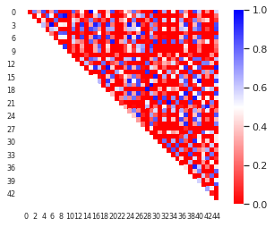
3.保留热图的上三角或下三角：（triu和tril对应上下三角）

 1 corr = np.corrcoef(tm_array)
 2 mask = np.zeros_like(corr)
 3 
 4 mask[np.tril_indices_from(mask)] = True
 5 with sns.axes_style("white"):
 6     ax = sns.heatmap(corr, mask=mask, vmax=1, vmin=0,cmap='bwr_r', square=True)
 7 ax.tick_params(labelsize=8) # y轴
 8 # 旋转轴刻度上文字方向的两种方法
 9 ax.set_yticklabels(ax.get_yticklabels(), rotation=0)
10 ax.set_xticklabels(ax.get_xticklabels(), rotation=0)
11 #plt.savefig('tm_array.png', dpi=300) #指定分辨率保存
12 plt.show()

4.将两个矩阵的上下三角分别取出并合并即可画出合并图：

1 up_rmsd=np.triu(rmsd_array, k=1)# Upper triangle of an array
2 lower_tm=np.tril(tm_array, k=-1)# Lower triangle of an array.
3 montage_array= up_rmsd+lower_tm
4  
5 print(montage_array)

[[ 0.     15.289  10.037  ... 10.173  18.827   7.309 ]
 [ 0.3905  0.     19.317  ... 19.324  24.559  12.865 ]
 [ 0.6914  0.3591  0.     ...  9.504  15.224  12.05  ]
 ...
 [ 0.4976  0.3587  0.531  ...  0.     14.592  12.491 ]
 [ 0.3588  0.2798  0.3791 ...  0.3962  0.     20.118 ]
 [ 0.6454  0.4366  0.4668 ...  0.476   0.3236  0.    ]]
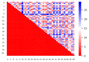
但是，我们的两个矩阵元素不是一个衡量标准：rmsd_array和tm_array的值范围分别为（0，25），（0，1）
如果不做处理画出来是这样的：

5，由上，需要先对rmsd_array的值做一下归一化：

 1 '''
 2 Tips：归一化处理normalization也可以自己用python写，这里为了方便就调用现成的包了
 3 def MaxMinNormalization(x,Max,Min):
 4     x = (x - Min) / (Max - Min);
 5     return x;
 6     '''
 7 from sklearn import preprocessing
 8 #归一化处理normalization
 9 min_max_scaler = preprocessing.MinMaxScaler()
10 rmsd_array_normal=min_max_scaler.fit_transform(rmsd_array)

up_rmsd=np.triu(rmsd_array_normal, k=1)# Upper triangle of an array
lower_tm=np.tril(tm_array, k=-1)# Lower triangle of an array.
montage_array= up_rmsd+lower_tm
 
print(montage_array)

[[0.         0.54586026 0.43536913 ... 0.44195847 0.71149994 0.29112563]
 [0.3905     0.         0.83790232 ... 0.8395169  0.92812063 0.51242731]
 [0.6914     0.3591     0.         ... 0.41289426 0.57533729 0.47996495]
 ...
 [0.4976     0.3587     0.531      ... 0.         0.55145308 0.49753047]
 [0.3588     0.2798     0.3791     ... 0.3962     0.         0.80132239]
 [0.6454     0.4366     0.4668     ... 0.476      0.3236     0.        ]]

6,将处理后的矩阵 montage_array重新画一下热图，就得到了想要的结果。

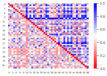
over!