For binary classification (+1, -1), if we classify correctly then (ycdot f = ycdot heta^Txgt0); otherwise (ycdot f = ycdot heta^Txlt0). Thus we have following loss functions:
- 0/1 loss
(min_ hetasum_i L_{0/1}( heta^Tx)). We define (L_{0/1}( heta^Tx) =1) if (ycdot f lt 0), and (=0) o.w. Non convex and very hard to optimize. - Hinge loss
Upper Bound of 0/1 loss. Approximate 0/1 loss by (min_ hetasum_i H( heta^Tx)). We define (H( heta^Tx) = max(0, 1 - ycdot f)). Apparently (H) is small if we classify correctly. - Logistic loss
(min_ heta sum_i log(1+exp(-ycdot heta^Tx))).
Fortunately, hinge loss, logistic loss and square loss are all convex functions. Convexity ensures global minimum and it's computationally appealing.
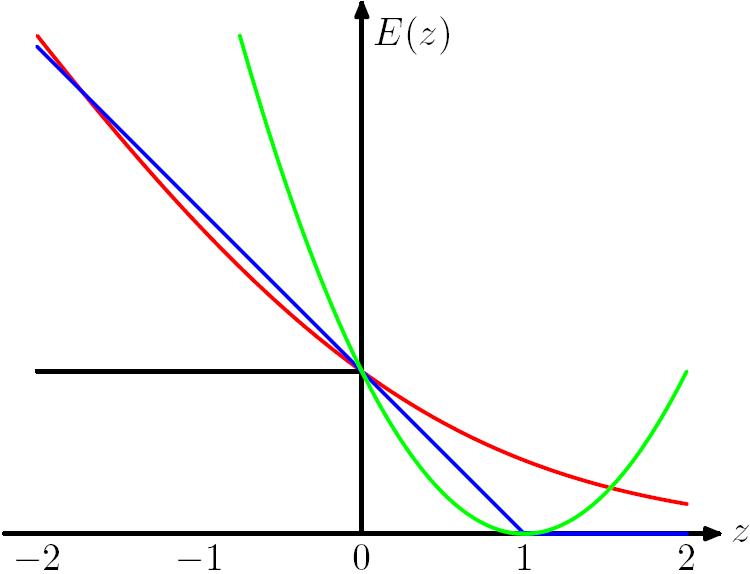
Figure 7.5 from Chris Bishop's PRML book. The Hinge Loss E(z) = max(0,1-z) is plotted in blue, the Log Loss in red, the Square Loss in green and the 0/1 error in black.
From the figure we can observe that the hard instance (near the boundary) will influence the loss function a lot so we need to make the model robust and can deal with the hard ones.
For binary classification we can unify the two cases (classify correctly or not) by (ycdot f), but for multi-class classification (0, 1, 2, ..., k) we cannot unify all the cases. So we use cross-entropy as the loss.
There exists a vivid example for transform the target function: If a noisy picture is given, and want to output the clean one. Here the clean one is hard to control so we can let the noise be the target function and wo should minimize the amplitude of the noise. Thus the problem becomes controllable.