科学计算和可视化（numpy及matplotlib学习笔记）

网上学习资料：https://2d.hep.com.cn/1865445/9

numpy库内容:

函数	描述
np.array([x,y,z],dtype=int)	从Python列表和元组创造数组
np.arange(x,y,i)	创建一个从x到y，步长为 i 的数组
np.linspace(x,y,n)	创建一个从x到y，等分成 n 个元素的数组
np.indices((m,n))	创建一个 m 行 n 列的矩阵
np.random.rand(m,n)	创建一个 m 行 n 列的随机数组
np.ones((m,n),dtype)	创建一个 m 行 n 列全为 1 的数组，dtype是数据类型
np.empty((m,n),dtype)	创建一个 m 行 n 列全为0的数组，dtype是数据类型

  实例（教材）：

 #e17.1HandDrawPic.py
 from PIL import Image
 import numpy as np
 vec_el = np.pi/2.2 # 光源的俯视角度，弧度值
 vec_az = np.pi/4. # 光源的方位角度，弧度值
 depth = 10. # (0-100)
 im = Image.open('fcity.jpg').convert('L')
 a = np.asarray(im).astype('float')
 grad = np.gradient(a) #取图像灰度的梯度值
 grad_x, grad_y = grad #分别取横纵图像梯度值
 grad_x = grad_x*depth/100.
 grad_y = grad_y*depth/100.
 dx = np.cos(vec_el)*np.cos(vec_az) #光源对x 轴的影响
 dy = np.cos(vec_el)*np.sin(vec_az) #光源对y 轴的影响
 dz = np.sin(vec_el) #光源对z 轴的影响
 A = np.sqrt(grad_x**2 + grad_y**2 + 1.)
 uni_x = grad_x/A
 uni_y = grad_y/A
 uni_z = 1./A
 a2 = 255*(dx*uni_x + dy*uni_y + dz*uni_z) #光源归一化
 a2 = a2.clip(0,255)
 im2 = Image.fromarray(a2.astype('uint8')) #重构图像
 im2.save('fcityHandDraw.jpg

matplotlib库主要内容：

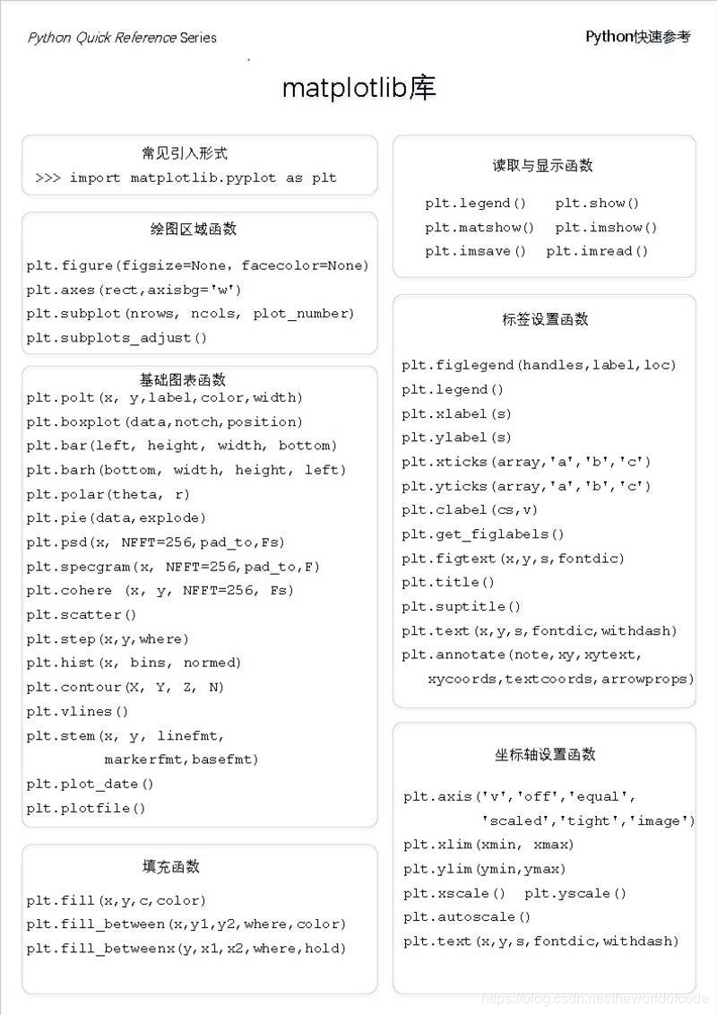
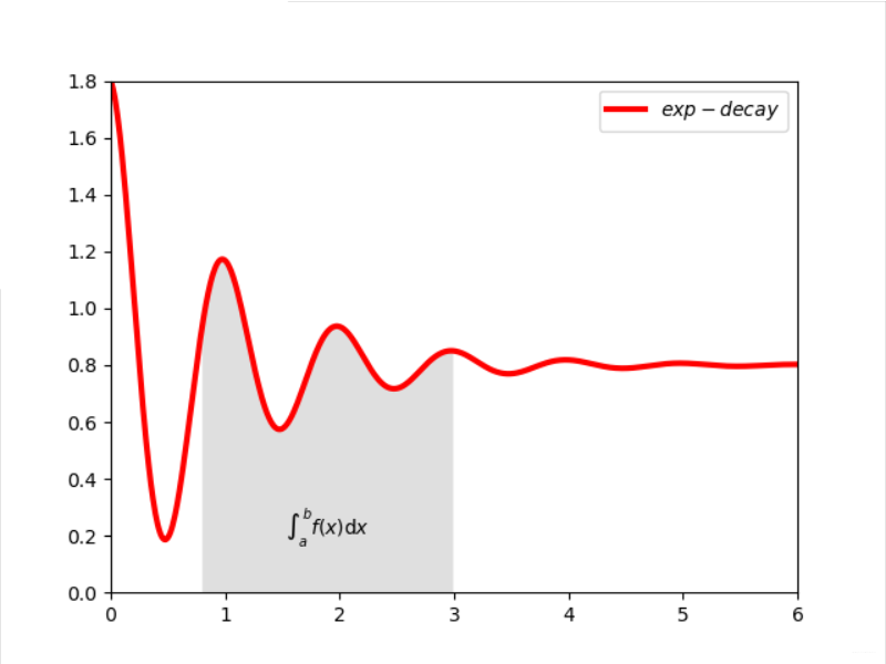
实例（教材）：带阴影的坐标系

import matplotlib.pyplot as plt
import numpy as np
x = np.linspace(0, 10, 1000)
y = np.cos(2*np.pi*x) * np.exp(-x)+0.8
plt.plot(x,y,'k',color='r',label="$exp-decay$",linewidth=3)
plt.axis([0,6,0,1.8])
ix = (x>0.8) & (x<3)
plt.fill_between(x, y ,0, where = ix, 
                         facecolor='grey', alpha=0.25)
plt.text(0.5*(0.8+3), 0.2, r"$int_a^b f(x)mathrm{d}x$",
                horizontalalignment='center')
plt.legend()
plt.show()

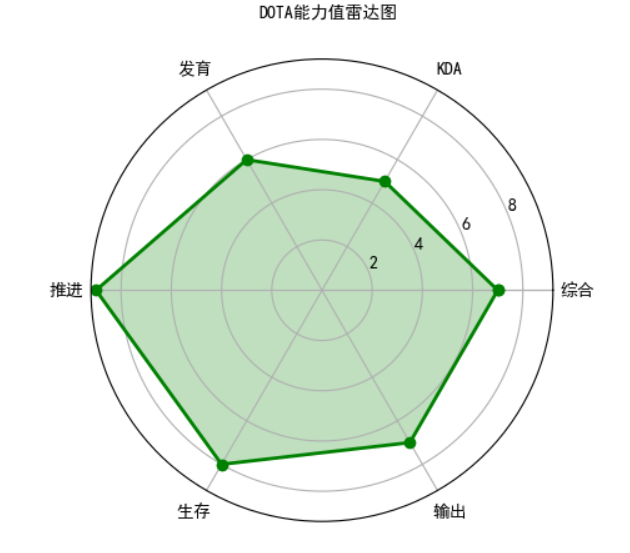
 实例（教材）：DOTA能力雷达图

#e19.1DrawRadar
import numpy as np
import matplotlib.pyplot as plt
import matplotlib
matplotlib.rcParams['font.family']='SimHei'
matplotlib.rcParams['font.sans-serif'] = ['SimHei']
labels = np.array(['综合', 'KDA', '发育', '推进', '生存','输出'])
nAttr = 6
data = np.array([7, 5, 6, 9, 8, 7]) #数据值
angles = np.linspace(0, 2*np.pi, nAttr, endpoint=False)
data = np.concatenate((data, [data[0]]))
angles = np.concatenate((angles, [angles[0]]))
fig = plt.figure(facecolor="white")
plt.subplot(111, polar=True)
plt.plot(angles,data,'bo-',color ='g',linewidth=2)
plt.fill(angles,data,facecolor='g',alpha=0.25)
plt.thetagrids(angles*180/np.pi, labels)
plt.figtext(0.52, 0.95, 'DOTA能力值雷达图', ha='center')
plt.grid(True)
plt.show()

 实例：python成绩雷达图

import numpy as np
import matplotlib.pyplot as plt
labels = np.array(['第二周','第三周','第四周','第五周','第六周'])
dataLenth =5
data = np.array([100,93.3,100,110,60])
angles = np.linspace(0, 2*np.pi, dataLenth, endpoint=False)
data = np.concatenate((data, [data[0]]))
angles = np.concatenate((angles, [angles[0]]))
fig = plt.figure()
ax = fig.add_subplot(111, polar=True)
ax.plot(angles, data, 'ro-', linewidth=2)
ax.set_thetagrids(angles * 180/np.pi, labels, fontproperties="SimHei")
ax.set_title("呆.的python成绩雷达图", va='bottom', fontproperties="SimHei")
ax.grid(True)
plt.show()

、