CNN卷积神经网络学习记录（1）

通过对斯坦福大学2017秋季，卷积神经网络的公开课CS231n，做以总结，辅助学习Tensorflow
地址：https://cs231n.github.io/convolutional-networks/

Convolutional Neural Networks（CNN）：

首先卷积神经网络和传统的神经网络类似都需要接受一些inputs，也拥有可以进行学习的weight和biases，他也有激励函数和loss函数等等

卷积神经网络的架构：

　　首先他也有input和output 的layers， input为数据输入层，output为结果输出层。

　　在图像识别领域，input代表了一系列的输入的图片，比如[32,32,3]就是32x32像素的3原色组成的彩色图片。

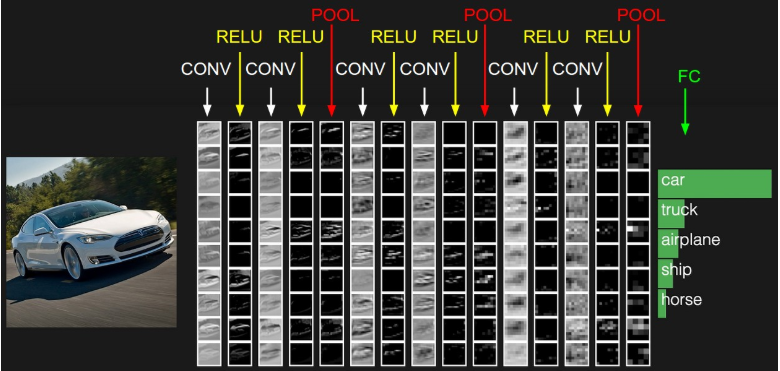
　　CONV layer，也就是卷积层，卷积层会计算连接到input区域的weight，会用到激励函数，举例结果可能是[32,32,12]如果我们设置了12个filter的话。

　　POOL layer，池层的主要作用是压缩input的大小，比如[16,16,12]

　　FC layer(fully-connected layer) 把像素等值转化为一个[1,1,10]的值（因为数字从0-9）得出结果

In this way, ConvNets transform the original image layer by layer from the original pixel values to the final class scores. Note that some layers contain parameters and other don’t. In particular, the CONV/FC layers perform transformations that are a function of not only the activations in the input volume, but also of the parameters (the weights and biases of the neurons). On the other hand, the RELU/POOL layers will implement a fixed function. The parameters in the CONV/FC layers will be trained with gradient descent so that the class scores that the ConvNet computes are consistent with the labels in the training set for each image.

流程图：

接下来做一下各个层的详细解释以及应用：

首先是卷积层(CONV) ：在卷积层中，当一个高维度的input传入时，比如3维的图片，仅仅会有一部分的神经元去进行连接，连接的区域就叫做，感知区域(receptive field)，拿图片举例，在连接过程中，width 和height是可以仅仅连接到感知区域的神经元，但是depth必须是全连接，举例说明，一个input是[32x32x3]，如果感知区域是[5x5]则卷积层的weight就为[5x5x3]也就是75个weights，加上一个bias。

如图：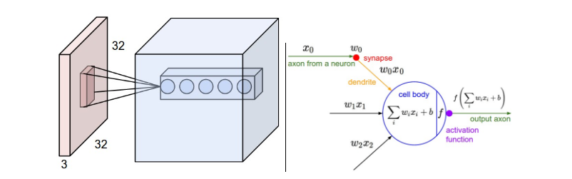

Spatial arrangement：我们解释了卷积层如何处理input，然后处理完input后，如果处理卷积层的output，这里有三个参数控制了输出的大小，depth（深度），stride（步长），zero-padding（补余）。

depth：代表了有多少个filter，也就是在一个相同的感知区域中，有多少个神经元，每个神经元分析不同的部分，比如颜色，轮廓，线条等等。

stride：步长，代表整个filter每次移动多少个像素。

zero-padding：用来保证输入和输出的width和height相同，用0来补充矩阵。

通过参数化，我们可以计算出输出的范围，假设输入size的值为(W)，卷积层感知区域的神经元数量为(F)，步长为(S)，zero-padding为(P)，则可以用 (W - F + 2P)/S + 1来算出输出的size。比如一个7x7 的输入，和3x3的感知区域，步长为1，padding为0，则通过公式可以得出output的size为5X5，如果步长为2，则output为3x3 =>(7 - 3 + 2x0)/ 2 + 1.

参数配置问题：比如(W - F + 2P)/S + 1 = (10 - 3 + 0)/2 + 1 = 4.5得出一个非Integer的值。这种情况下，需要zero padding来填补，以及控制步长，否则神经网络会报错。

参数共享：是用在卷积层用来控制参数，如果一组参数可以高效的进行计算，那在另一个位置，他也拥有相同的能力。换句话说，在一个[55x55x96]的volumn中，有96个深度，每层深度为[55x55]都使用相同的weight和bias，在back propagatin的过程中，每个depth slice只需要update对应的weight。比如在机器学习的过程中，在像素矩阵中检测到一个水平的线，那这组weight和bias可以用在其他可检测到水平线的参数中去。 Tips：有时候参数共享并不一定实用，因为实用的情况是假设数据组有很多相似点，如果说完全不同的图片进行机器学习的话，就应当学习每个slice。

用Python的Numpy来表示之前的概念：

一个depth column在位置(x,y) 可以表示为X[x,y,:]

一个depth slice，在深度为d的一层可以表示为X[:,:,d]

假设一个输入为x.shape(11,11,4)，zero-padding为0，感知区size =>F为5，步长S为2，根据之前的公式可以算出(11-5)/2+1 = 4，也就是output为4X4，我们把输出标记为V，则举例：

V[0,0,0] = np.sum(X[:5,:5,:] * W0) + b0
V[1,0,0] = np.sum(X[2:7,:5,:] * W0) + b0
V[2,0,0] = np.sum(X[4:9,:5,:] * W0) + b0
V[3,0,0] = np.sum(X[6:11,:5,:] * W0) + b0

当进到depth为1的时候，w，b的参数亦随之改变：

V[0,0,1] = np.sum(X[:5,:5,:] * W1) + b1
V[1,0,1] = np.sum(X[2:7,:5,:] * W1) + b1
V[2,0,1] = np.sum(X[4:9,:5,:] * W1) + b1
V[3,0,1] = np.sum(X[6:11,:5,:] * W1) + b1
V[0,1,1] = np.sum(X[:5,2:7,:] * W1) + b1 (example of going along y)
V[2,3,1] = np.sum(X[4:9,6:11,:] * W1) + b1 (or along both)

待续。

2018/7/5:

最近都在工作很忙，没时间更新博客，但是学习的脚步从未停下，放一张很形象的cnn图

再插一段cnn 的 MINST数字识别代码

import tensorflow as tf
import numpy as np
import matplotlib.pyplot as plt
from tensorflow.examples.tutorials.mnist import input_data

mnist = input_data.read_data_sets('MNIST_data',one_hot = True)


def compute_accuracy(v_xs, v_ys):
    global prediction
    y_pre = sess.run(prediction, feed_dict={xs: v_xs})
    correct_prediction = tf.equal(tf.argmax(y_pre, 1), tf.argmax(v_ys, 1))
    accuracy = tf.reduce_mean(tf.cast(correct_prediction, tf.float32))
    result = sess.run(accuracy, feed_dict={xs: v_xs, ys: v_ys})
    return result


def weight_variable(shape):
    initial = tf.truncated_normal(shape, stddev=0.1)
    return tf.Variable(initial)


def bias_variable(shape):
    initial = tf.constant(0.1, shape=shape)
    return tf.Variable(initial)


def conv2d(x, W):
    #strides[1, x_move, y_move, 1]
    return tf.nn.conv2d(x, W, strides=[1,1,1,1], padding='SAME')


def max_pool_2x2(x):
    return tf.nn.max_pool(x, ksize=[1,2,2,1], strides=[1,2,2,1], padding='SAME')


xs = tf.placeholder(tf.float32, [None, 784])/255.
ys = tf.placeholder(tf.float32, [None, 10])
keep_prob = tf.placeholder(tf.float32)
x_image = tf.reshape(xs,[-1,28,28,1])


##layers##
# conv1
W_conv1 = weight_variable([5, 5, 1, 32])
b_conv1 = bias_variable([32])
h_conv1 = tf.nn.relu(conv2d(x_image,W_conv1) + b_conv1)# output size 28X28X32, 因为padding，所以并没有减少input层
h_pool1 = max_pool_2x2(h_conv1)# output size 14X14X32

#conv2
W_conv2 = weight_variable([5, 5, 32, 64]) #传入为32，传出为64
b_conv2 = bias_variable([64])
h_conv2 = tf.nn.relu(conv2d(h_pool1,W_conv2) + b_conv2)# output size 14X14X64, 因为padding，所以并没有减少input层
h_pool2 = max_pool_2x2(h_conv2)# output size 7X7X64

#func1 layer
W_fc1 = weight_variable([7*7*64, 1024])
b_fc1 = bias_variable([1024])

h_pool2_falt = tf.reshape(h_pool2, [-1, 7*7*64])
h_fc1= tf.nn.relu(tf.matmul(h_pool2_falt, W_fc1) + b_fc1)
h_fc1_drop = tf.nn.dropout(h_fc1, keep_prob)
#func2 layer
W_fc2 = weight_variable([1024, 10])
b_fc2 = bias_variable([10])
prediction= tf.nn.softmax(tf.matmul(h_fc1_drop, W_fc2) + b_fc2)
##layers##

#loss
cross_entropy = tf.reduce_mean(-tf.reduce_sum(ys * tf.log(prediction), reduction_indices=[1]))
train_step = tf.train.AdamOptimizer(1e-4).minimize(cross_entropy)

sess = tf.Session()
sess.run(tf.global_variables_initializer())

for i in range(10000):
    batch_xs, batch_ys = mnist.train.next_batch(100)
    sess.run(train_step, feed_dict={xs: batch_xs, ys: batch_ys, keep_prob: 0.5})
    if i % 50 == 0:
        print(compute_accuracy(
            mnist.test.images[:1000], mnist.test.labels[:1000]
        ))