1.引言
一个多层感知机(Multi-Layer Perceptron,MLP)可以看做是,在逻辑回归分类器的中间加了非线性转换的隐层,这种转换把数据映射到一个线性可分的空间。一个单隐层的MLP就可以达到全局最优。
2.模型
一个单隐层的MLP可以表示如下:

一个隐层的MLP是一个函数:$f:R^{D} ightarrow R^{L}$,其中 $D$ 是输入向量 $x$ 的大小,$L$是输出向量 $f(x)$ 的大小:
$f(x)=G(b^{(2)}+W^{(2)}(s(b^{(1)}+W^{(1)}))),$
向量$h(x)=s(b^{(1)}+W^{(1)})$构成了隐层,$W^{(1)}in R^{D imes D_{h}}$ 是连接输入和隐层的权重矩阵,激活函数$s$可以是 $tanh(a)=(e^{a}-e^{-a})/(e^{a}+e^{-a})$ 或者 $sigmoid(a)=1/(1+e^{-a})$,但是前者通常会训练比较快。
在输出层得到:$o(x)=G(b^{(2)}+W^{(2)}h(x))$
为了训练MLP,所有参数 $ heta={W^{(2)},b^{(2)},W^{(1)},b^{ ext{(1)}}}.$ 用随机梯度下降法训练,参数的求导用反向传播算法来求。这里在顶层分类的时候用到了前面的逻辑回归的代码:
Python学习笔记之逻辑回归.
3.从逻辑回归到MLP
这里以单隐层MLP为例,当把数据由输入层映射到隐层之后,再加上一个逻辑回归层就构成了MLP.
 1 class HiddenLayer(object):
 2     def __init__(self, rng, input, n_in, n_out, W=None, b=None,
 3                  activation=T.tanh):
 4         """
 5         Typical hidden layer of a MLP: units are fully-connected and have
 6         sigmoidal activation function. Weight matrix W is of shape (n_in,n_out)
 7         and the bias vector b is of shape (n_out,).
 8
 9         NOTE : The nonlinearity used here is tanh
10
11         Hidden unit activation is given by: tanh(dot(input,W) + b)
12
13         :type rng: numpy.random.RandomState
14         :param rng: a random number generator used to initialize weights
15
16         :type input: theano.tensor.dmatrix
17         :param input: a symbolic tensor of shape (n_examples, n_in)
18
19         :type n_in: int
20         :param n_in: dimensionality of input
21
22         :type n_out: int
23         :param n_out: number of hidden units
24
25         :type activation: theano.Op or function
26         :param activation: Non linearity to be applied in the hidden
27                            layer
28         """
29         self.input = input
权重的初始化依赖于激活函数,根据[Xavier10]证明显示,对于$tanh$激活函数,权重初始值应该从$[-sqrt{frac{6}{fan_{in}+fan_{out}}},sqrt{frac{6}{fan_{in}+fan_{out}}}]$区间内均匀采样得到,其中 $fan_{in}$ 是第$(i-1)$ 层的单元数量,$fan_{out}$ 是第 $i$ 层的单元数量,对于sigmoid函数,采样区间应该变为 $[-4sqrt{frac{6}{fan_{in}+fan_{out}}},4sqrt{frac{6}{fan_{in}+fan_{out}}}]$.这种初始化方式能保证在训练的初始阶段,通过激活函数能够使得信息有效地向上和向下传播。
 1 if W is None:
 2             W_values = numpy.asarray(
 3                 rng.uniform(
 4                     # 随机数位于[low,high)区间
 5                     low=-numpy.sqrt(6. / (n_in + n_out)),
 6                     high=numpy.sqrt(6. / (n_in + n_out)),
 7                     size=(n_in, n_out)
 8                 ),
 9                 # 类型设为 floatX 是为了在GPU上运行
10                 dtype=theano.config.floatX
11             )
12             # 如果激活函数是 sigmoid,权重初始化要变大
13             if activation == theano.tensor.nnet.sigmoid:
14                 W_values *= 4
15             # borrow = True 表示数据执行浅拷贝,增加效率
16             W = theano.shared(value=W_values, name='W', borrow=True)
17
18         if b is None:
19             b_values = numpy.zeros((n_out,), dtype=theano.config.floatX)
20             b = theano.shared(value=b_values, name='b', borrow=True)
21
22         self.W = W
23         self.b = b
24
25         lin_output = T.dot(input, self.W) + self.b
26         self.output = (
27             lin_output if activation is None
28             else activation(lin_output)
29         )
30         # parameters of the model
31         self.params = [self.W, self.b]
在上面两步的基础上构建MLP:
 1 class MLP(object):
 2     """Multi-Layer Perceptron Class
 3
 4     A multilayer perceptron is a feedforward artificial neural network model
 5     that has one layer or more of hidden units and nonlinear activations.
 6     Intermediate layers usually have as activation function tanh or the
 7     sigmoid function (defined here by a ``HiddenLayer`` class)  while the
 8     top layer is a softamx layer (defined here by a ``LogisticRegression``
 9     class).
10     """
11
12     def __init__(self, rng, input, n_in, n_hidden, n_out):
13         """Initialize the parameters for the multilayer perceptron
14
15         :type rng: numpy.random.RandomState
16         :param rng: a random number generator used to initialize weights
17
18         :type input: theano.tensor.TensorType
19         :param input: symbolic variable that describes the input of the
20         architecture (one minibatch)
21
22         :type n_in: int
23         :param n_in: number of input units, the dimension of the space in
24         which the datapoints lie
25
26         :type n_hidden: int
27         :param n_hidden: number of hidden units
28
29         :type n_out: int
30         :param n_out: number of output units, the dimension of the space in
31         which the labels lie
32
33         """
34
35         # Since we are dealing with a one hidden layer MLP, this will translate
36         # into a HiddenLayer with a tanh activation function connected to the
37         # LogisticRegression layer; the activation function can be replaced by
38         # sigmoid or any other nonlinear function
39         self.hiddenLayer = HiddenLayer(
40             rng=rng,
41             input=input,
42             n_in=n_in,
43             n_out=n_hidden,
44             activation=T.tanh
45         )
46
47         # The logistic regression layer gets as input the hidden units
48         # of the hidden layer
49         self.logRegressionLayer = LogisticRegression(
50             input=self.hiddenLayer.output,
51             n_in=n_hidden,
52             n_out=n_out
53         )
为了防止过拟合,这里加上 L1 和 L2 正则项,即计算权重 $W^{(1)},W^{(2)}$ 的1范数和2范数:
 1   # L1 norm ; one regularization option is to enforce L1 norm to
 2         # be small
 3         self.L1 = (
 4             abs(self.hiddenLayer.W).sum()
 5             + abs(self.logRegressionLayer.W).sum()
 6         )
 7
 8         # square of L2 norm ; one regularization option is to enforce
 9         # square of L2 norm to be small
10         self.L2_sqr = (
11             (self.hiddenLayer.W ** 2).sum()
12             + (self.logRegressionLayer.W ** 2).sum()
13         )
14
15         # negative log likelihood of the MLP is given by the negative
16         # log likelihood of the output of the model, computed in the
17         # logistic regression layer
18         self.negative_log_likelihood = (
19             self.logRegressionLayer.negative_log_likelihood
20         )
21         # same holds for the function computing the number of errors
22         self.errors = self.logRegressionLayer.errors
23
24         # the parameters of the model are the parameters of the two layer it is
25         # made out of
26         self.params = self.hiddenLayer.params + self.logRegressionLayer.params
似然函数的值加上正则项构成损失函数:
1 # the cost we minimize during training is the negative log likelihood of
2     # the model plus the regularization terms (L1 and L2); cost is expressed
3     # here symbolically
4     cost = (
5         classifier.negative_log_likelihood(y)
6         + L1_reg * classifier.L1
7         + L2_reg * classifier.L2_sqr
8     )
4.Minist识别测试


  1 """
  2 This tutorial introduces the multilayer perceptron using Theano.
  3
  4  A multilayer perceptron is a logistic regressor where
  5 instead of feeding the input to the logistic regression you insert a
  6 intermediate layer, called the hidden layer, that has a nonlinear
  7 activation function (usually tanh or sigmoid) . One can use many such
  8 hidden layers making the architecture deep. The tutorial will also tackle
  9 the problem of MNIST digit classification.
 10
 11 .. math::
 12
 13     f(x) = G( b^{(2)} + W^{(2)}( s( b^{(1)} + W^{(1)} x))),
 14
 15 References:
 16
 17     - textbooks: "Pattern Recognition and Machine Learning" -
 18                  Christopher M. Bishop, section 5
 19
 20 """
 21 __docformat__ = 'restructedtext en'
 22
 23
 24 import os
 25 import sys
 26 import time
 27
 28 import numpy
 29
 30 import theano
 31 import theano.tensor as T
 32
 33
 34 from logistic_sgd import LogisticRegression, load_data
 35
 36
 37 # start-snippet-1
 38 class HiddenLayer(object):
 39     def __init__(self, rng, input, n_in, n_out, W=None, b=None,
 40                  activation=T.tanh):
 41         """
 42         Typical hidden layer of a MLP: units are fully-connected and have
 43         sigmoidal activation function. Weight matrix W is of shape (n_in,n_out)
 44         and the bias vector b is of shape (n_out,).
 45
 46         NOTE : The nonlinearity used here is tanh
 47
 48         Hidden unit activation is given by: tanh(dot(input,W) + b)
 49
 50         :type rng: numpy.random.RandomState
 51         :param rng: a random number generator used to initialize weights
 52
 53         :type input: theano.tensor.dmatrix
 54         :param input: a symbolic tensor of shape (n_examples, n_in)
 55
 56         :type n_in: int
 57         :param n_in: dimensionality of input
 58
 59         :type n_out: int
 60         :param n_out: number of hidden units
 61
 62         :type activation: theano.Op or function
 63         :param activation: Non linearity to be applied in the hidden
 64                            layer
 65         """
 66         self.input = input
 67         # end-snippet-1
 68
 69         # `W` is initialized with `W_values` which is uniformely sampled
 70         # from sqrt(-6./(n_in+n_hidden)) and sqrt(6./(n_in+n_hidden))
 71         # for tanh activation function
 72         # the output of uniform if converted using asarray to dtype
 73         # theano.config.floatX so that the code is runable on GPU
 74         # Note : optimal initialization of weights is dependent on the
 75         #        activation function used (among other things).
 76         #        For example, results presented in [Xavier10] suggest that you
 77         #        should use 4 times larger initial weights for sigmoid
 78         #        compared to tanh
 79         #        We have no info for other function, so we use the same as
 80         #        tanh.
 81         if W is None:
 82             W_values = numpy.asarray(
 83                 rng.uniform(
 84                     # 随机数位于[low,high)区间
 85                     low=-numpy.sqrt(6. / (n_in + n_out)),
 86                     high=numpy.sqrt(6. / (n_in + n_out)),
 87                     size=(n_in, n_out)
 88                 ),
 89                 # 类型设为 floatX 是为了在GPU上运行
 90                 dtype=theano.config.floatX
 91             )
 92             # 如果激活函数是 sigmoid,权重初始化要变大
 93             if activation == theano.tensor.nnet.sigmoid:
 94                 W_values *= 4
 95             # borrow = True 表示数据执行浅拷贝,增加效率
 96             W = theano.shared(value=W_values, name='W', borrow=True)
 97
 98         if b is None:
 99             b_values = numpy.zeros((n_out,), dtype=theano.config.floatX)
100             b = theano.shared(value=b_values, name='b', borrow=True)
101
102         self.W = W
103         self.b = b
104
105         lin_output = T.dot(input, self.W) + self.b
106         self.output = (
107             lin_output if activation is None
108             else activation(lin_output)
109         )
110         # parameters of the model
111         self.params = [self.W, self.b]
112
113
114 # start-snippet-2
115 class MLP(object):
116     """Multi-Layer Perceptron Class
117
118     A multilayer perceptron is a feedforward artificial neural network model
119     that has one layer or more of hidden units and nonlinear activations.
120     Intermediate layers usually have as activation function tanh or the
121     sigmoid function (defined here by a ``HiddenLayer`` class)  while the
122     top layer is a softamx layer (defined here by a ``LogisticRegression``
123     class).
124     """
125
126     def __init__(self, rng, input, n_in, n_hidden, n_out):
127         """Initialize the parameters for the multilayer perceptron
128
129         :type rng: numpy.random.RandomState
130         :param rng: a random number generator used to initialize weights
131
132         :type input: theano.tensor.TensorType
133         :param input: symbolic variable that describes the input of the
134         architecture (one minibatch)
135
136         :type n_in: int
137         :param n_in: number of input units, the dimension of the space in
138         which the datapoints lie
139
140         :type n_hidden: int
141         :param n_hidden: number of hidden units
142
143         :type n_out: int
144         :param n_out: number of output units, the dimension of the space in
145         which the labels lie
146
147         """
148
149         # Since we are dealing with a one hidden layer MLP, this will translate
150         # into a HiddenLayer with a tanh activation function connected to the
151         # LogisticRegression layer; the activation function can be replaced by
152         # sigmoid or any other nonlinear function
153         self.hiddenLayer = HiddenLayer(
154             rng=rng,
155             input=input,
156             n_in=n_in,
157             n_out=n_hidden,
158             activation=T.tanh
159         )
160
161         # The logistic regression layer gets as input the hidden units
162         # of the hidden layer
163         self.logRegressionLayer = LogisticRegression(
164             input=self.hiddenLayer.output,
165             n_in=n_hidden,
166             n_out=n_out
167         )
168         # end-snippet-2 start-snippet-3
169         # L1 norm ; one regularization option is to enforce L1 norm to
170         # be small
171         self.L1 = (
172             abs(self.hiddenLayer.W).sum()
173             + abs(self.logRegressionLayer.W).sum()
174         )
175
176         # square of L2 norm ; one regularization option is to enforce
177         # square of L2 norm to be small
178         self.L2_sqr = (
179             (self.hiddenLayer.W ** 2).sum()
180             + (self.logRegressionLayer.W ** 2).sum()
181         )
182
183         # negative log likelihood of the MLP is given by the negative
184         # log likelihood of the output of the model, computed in the
185         # logistic regression layer
186         self.negative_log_likelihood = (
187             self.logRegressionLayer.negative_log_likelihood
188         )
189         # same holds for the function computing the number of errors
190         self.errors = self.logRegressionLayer.errors
191
192         # the parameters of the model are the parameters of the two layer it is
193         # made out of
194         self.params = self.hiddenLayer.params + self.logRegressionLayer.params
195         # end-snippet-3
196
197
198 def test_mlp(learning_rate=0.01, L1_reg=0.00, L2_reg=0.0001, n_epochs=1000,
199              dataset='mnist.pkl.gz', batch_size=20, n_hidden=500):
200     """
201     Demonstrate stochastic gradient descent optimization for a multilayer
202     perceptron
203
204     This is demonstrated on MNIST.
205
206     :type learning_rate: float
207     :param learning_rate: learning rate used (factor for the stochastic
208     gradient
209
210     :type L1_reg: float
211     :param L1_reg: L1-norm's weight when added to the cost (see
212     regularization)
213
214     :type L2_reg: float
215     :param L2_reg: L2-norm's weight when added to the cost (see
216     regularization)
217
218     :type n_epochs: int
219     :param n_epochs: maximal number of epochs to run the optimizer
220
221     :type dataset: string
222     :param dataset: the path of the MNIST dataset file from
223                  http://www.iro.umontreal.ca/~lisa/deep/data/mnist/mnist.pkl.gz
224
225
226    """
227     datasets = load_data(dataset)
228
229     train_set_x, train_set_y = datasets[0]
230     valid_set_x, valid_set_y = datasets[1]
231     test_set_x, test_set_y = datasets[2]
232
233     # compute number of minibatches for training, validation and testing
234     n_train_batches = train_set_x.get_value(borrow=True).shape[0] / batch_size
235     n_valid_batches = valid_set_x.get_value(borrow=True).shape[0] / batch_size
236     n_test_batches = test_set_x.get_value(borrow=True).shape[0] / batch_size
237
238     ######################
239     # BUILD ACTUAL MODEL #
240     ######################
241     print '... building the model'
242
243     # allocate symbolic variables for the data
244     index = T.lscalar()  # index to a [mini]batch
245     x = T.matrix('x')  # the data is presented as rasterized images
246     y = T.ivector('y')  # the labels are presented as 1D vector of
247                         # [int] labels
248
249     rng = numpy.random.RandomState(1234)
250
251     # construct the MLP class
252     classifier = MLP(
253         rng=rng,
254         input=x,
255         n_in=28 * 28,
256         n_hidden=n_hidden,
257         n_out=10
258     )
259
260     # start-snippet-4
261     # the cost we minimize during training is the negative log likelihood of
262     # the model plus the regularization terms (L1 and L2); cost is expressed
263     # here symbolically
264     cost = (
265         classifier.negative_log_likelihood(y)
266         + L1_reg * classifier.L1
267         + L2_reg * classifier.L2_sqr
268     )
269     # end-snippet-4
270
271     # compiling a Theano function that computes the mistakes that are made
272     # by the model on a minibatch
273     test_model = theano.function(
274         inputs=[index],
275         outputs=classifier.errors(y),
276         givens={
277             x: test_set_x[index * batch_size:(index + 1) * batch_size],
278             y: test_set_y[index * batch_size:(index + 1) * batch_size]
279         }
280     )
281
282     validate_model = theano.function(
283         inputs=[index],
284         outputs=classifier.errors(y),
285         givens={
286             x: valid_set_x[index * batch_size:(index + 1) * batch_size],
287             y: valid_set_y[index * batch_size:(index + 1) * batch_size]
288         }
289     )
290
291     # start-snippet-5
292     # compute the gradient of cost with respect to theta (sotred in params)
293     # the resulting gradients will be stored in a list gparams
294     gparams = [T.grad(cost, param) for param in classifier.params]
295
296     # specify how to update the parameters of the model as a list of
297     # (variable, update expression) pairs
298
299     # given two list the zip A = [a1, a2, a3, a4] and B = [b1, b2, b3, b4] of
300     # same length, zip generates a list C of same size, where each element
301     # is a pair formed from the two lists :
302     #    C = [(a1, b1), (a2, b2), (a3, b3), (a4, b4)]
303     updates = [
304         (param, param - learning_rate * gparam)
305         for param, gparam in zip(classifier.params, gparams)
306     ]
307
308     # compiling a Theano function `train_model` that returns the cost, but
309     # in the same time updates the parameter of the model based on the rules
310     # defined in `updates`
311     train_model = theano.function(
312         inputs=[index],
313         outputs=cost,
314         updates=updates,
315         givens={
316             x: train_set_x[index * batch_size: (index + 1) * batch_size],
317             y: train_set_y[index * batch_size: (index + 1) * batch_size]
318         }
319     )
320     # end-snippet-5
321
322     ###############
323     # TRAIN MODEL #
324     ###############
325     print '... training'
326
327     # early-stopping parameters
328     patience = 10000  # look as this many examples regardless
329     patience_increase = 2  # wait this much longer when a new best is
330                            # found
331     improvement_threshold = 0.995  # a relative improvement of this much is
332                                    # considered significant
333     validation_frequency = min(n_train_batches, patience / 2)
334                                   # go through this many
335                                   # minibatche before checking the network
336                                   # on the validation set; in this case we
337                                   # check every epoch
338
339     best_validation_loss = numpy.inf
340     best_iter = 0
341     test_score = 0.
342     start_time = time.clock()
343
344     epoch = 0
345     done_looping = False
346     # 迭代 n_epochs 次,每次迭代都将遍历训练集所有样本
347     while (epoch < n_epochs) and (not done_looping):
348         epoch = epoch + 1
349         for minibatch_index in xrange(n_train_batches):
350
351             minibatch_avg_cost = train_model(minibatch_index)
352             # iteration number
353             iter = (epoch - 1) * n_train_batches + minibatch_index
354
355             # 训练一定的样本之后才进行交叉验证
356             if (iter + 1) % validation_frequency == 0:
357                 # compute zero-one loss on validation set
358                 validation_losses = [validate_model(i) for i
359                                      in xrange(n_valid_batches)]
360                 this_validation_loss = numpy.mean(validation_losses)
361
362                 print(
363                     'epoch %i, minibatch %i/%i, validation error %f %%' %
364                     (
365                         epoch,
366                         minibatch_index + 1,
367                         n_train_batches,
368                         this_validation_loss * 100.
369                     )
370                 )
371
372                 # if we got the best validation score until now
373                 # 如果交叉验证的误差比当前最小的误差还小,就在测试集上测试
374                 if this_validation_loss < best_validation_loss:
375                     # improve patience if loss improvement is good enough
376                     # 如果改善很多,就在本次迭代中多训练一定数量的样本
377                     if (
378                         this_validation_loss < best_validation_loss *
379                         improvement_threshold
380                     ):
381                         patience = max(patience, iter * patience_increase)
382
383                     # 记录最小的交叉验证误差和相应的迭代数
384                     best_validation_loss = this_validation_loss
385                     best_iter = iter
386
387                     # test it on the test set
388                     test_losses = [test_model(i) for i
389                                    in xrange(n_test_batches)]
390                     test_score = numpy.mean(test_losses)
391
392                     print(('     epoch %i, minibatch %i/%i, test error of '
393                            'best model %f %%') %
394                           (epoch, minibatch_index + 1, n_train_batches,
395                            test_score * 100.))
396             # 训练样本数超过 patience,即停止
397             if patience <= iter:
398                 done_looping = True
399                 break
400
401     end_time = time.clock()
402     print(('Optimization complete. Best validation score of %f %% '
403            'obtained at iteration %i, with test performance %f %%') %
404           (best_validation_loss * 100., best_iter + 1, test_score * 100.))
405     print >> sys.stderr, ('The code for file ' +
406                           os.path.split(__file__)[1] +
407                           ' ran for %.2fm' % ((end_time - start_time) / 60.))
408
409
410 if __name__ == '__main__':
411     test_mlp()
关于上面代码中的交叉验证:只有训练结果的交叉验证结果比上一次交叉验证结果好,才在测试集上进行测试!
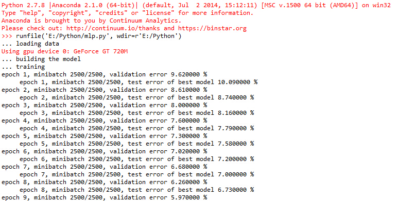
训练过程截图:
学习内容来源: