在很多情况下,我们要处理的数据的维度很高,需要提取主要的特征进行分析这就是PCA(主成分分析),白化是为了减少各个特征之间的冗余,因为在许多自然数据中,各个特征之间往往存在着一种关联,为了减少特征之间的关联,需要用到所谓的白化(whitening).
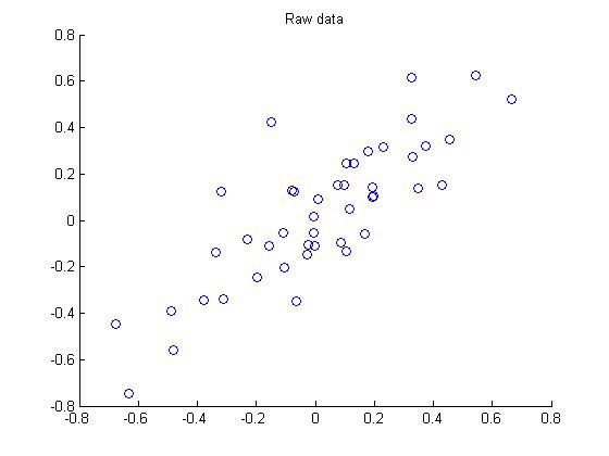
首先下载数据pcaData.rar,下面要对这里面包含的45个2维样本点进行PAC和白化处理,数据中每一列代表一个样本点。
第一步 画出原始数据:
第二步:执行PCA,找到数据变化最大的方向:

第三步:将原始数据投射到上面找的两个方向上:

第四步:降维,此例中把数据由2维降维到1维,画出降维后的数据:

第五步:PCA白化处理:

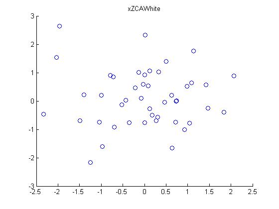
第六步:ZCA白化处理:
下面是程序matlab源代码:
  1 close all;clear all;clc;
  2
  3 %%================================================================
  4 %% Step 0: Load data
  5 %  We have provided the code to load data from pcaData.txt into x.
  6 %  x is a 2 * 45 matrix, where the kth column x(:,k) corresponds to
  7 %  the kth data point.Here we provide the code to load natural image data into x.
  8 %  You do not need to change the code below.
  9
 10 x = load('pcaData.txt','-ascii');
 11 figure(1);
 12 scatter(x(1, :), x(2, :));
 13 title('Raw data');
 14
 15
 16 %%================================================================
 17 %% Step 1a: Implement PCA to obtain U
 18 %  Implement PCA to obtain the rotation matrix U, which is the eigenbasis
 19 %  sigma.
 20
 21 % -------------------- YOUR CODE HERE --------------------
 22 u = zeros(size(x, 1)); % You need to compute this
 23
 24 sigma = x * x'/ size(x, 2);
 25 [u,S,V] = svd(sigma);
 26
 27
 28
 29 % --------------------------------------------------------
 30 hold on
 31 plot([0 u(1,1)], [0 u(2,1)]);
 32 plot([0 u(1,2)], [0 u(2,2)]);
 33 scatter(x(1, :), x(2, :));
 34 hold off
 35
 36 %%================================================================
 37 %% Step 1b: Compute xRot, the projection on to the eigenbasis
 38 %  Now, compute xRot by projecting the data on to the basis defined
 39 %  by U. Visualize the points by performing a scatter plot.
 40
 41 % -------------------- YOUR CODE HERE --------------------
 42 xRot = zeros(size(x)); % You need to compute this
 43 xRot = u' * x;
 44
 45 % --------------------------------------------------------
 46
 47 % Visualise the covariance matrix. You should see a line across the
 48 % diagonal against a blue background.
 49 figure(2);
 50 scatter(xRot(1, :), xRot(2, :));
 51 title('xRot');
 52
 53 %%================================================================
 54 %% Step 2: Reduce the number of dimensions from 2 to 1.
 55 %  Compute xRot again (this time projecting to 1 dimension).
 56 %  Then, compute xHat by projecting the xRot back onto the original axes
 57 %  to see the effect of dimension reduction
 58
 59 % -------------------- YOUR CODE HERE --------------------
 60 k = 1; % Use k = 1 and project the data onto the first eigenbasis
 61 xHat = zeros(size(x)); % You need to compute this
 62 z = u(:, 1:k)' * x;
 63 xHat = u(:,1:k) * z;
 64
 65 % --------------------------------------------------------
 66 figure(3);
 67 scatter(xHat(1, :), xHat(2, :));
 68 title('xHat');
 69
 70
 71 %%================================================================
 72 %% Step 3: PCA Whitening
 73 %  Complute xPCAWhite and plot the results.
 74
 75 epsilon = 1e-5;
 76 % -------------------- YOUR CODE HERE --------------------
 77 xPCAWhite = zeros(size(x)); % You need to compute this
 78
 79 xPCAWhite = diag(1 ./ sqrt(diag(S) + epsilon)) * xRot;
 80
 81
 82
 83 % --------------------------------------------------------
 84 figure(4);
 85 scatter(xPCAWhite(1, :), xPCAWhite(2, :));
 86 title('xPCAWhite');
 87
 88 %%================================================================
 89 %% Step 3: ZCA Whitening
 90 %  Complute xZCAWhite and plot the results.
 91
 92 % -------------------- YOUR CODE HERE --------------------
 93 xZCAWhite = zeros(size(x)); % You need to compute this
 94
 95 xZCAWhite = u * xPCAWhite;
 96 % --------------------------------------------------------
 97 figure(5);
 98 scatter(xZCAWhite(1, :), xZCAWhite(2, :));
 99 title('xZCAWhite');
100
101 %% Congratulations! When you have reached this point, you are done!
102 %  You can now move onto the next PCA exercise. :)