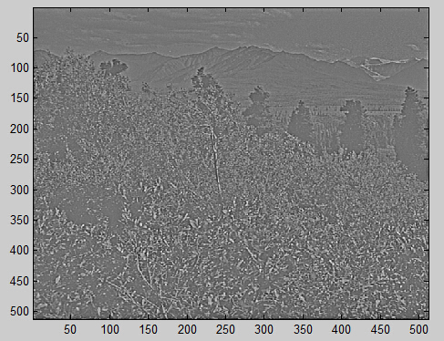
从10幅图像中采样出10000幅小图像块,每个小图像块大小是8*8,利用采样出的图像作为样本学习,利用LBFGS进行优化.
下面是对10幅图像白化之后的结果:
train.m
%% CS294A/CS294W Programming Assignment Starter Code
% Instructions
% ------------
%
% This file contains code that helps you get started on the
% programming assignment. You will need to complete the code in sampleIMAGES.m,
% sparseAutoencoderCost.m and computeNumericalGradient.m.
% For the purpose of completing the assignment, you do not need to
% change the code in this file.
%
%%======================================================================
%% STEP 0: Here we provide the relevant parameters values that will
% allow your sparse autoencoder to get good filters; you do not need to
% change the parameters below.
clear all;clc;
visibleSize = 8*8; % number of input units
hiddenSize = 25; % number of hidden units
sparsityParam = 0.01; % desired average activation of the hidden units.
% (This was denoted by the Greek alphabet rho, which looks like a lower-case "p",
% in the lecture notes).
lambda = 0.0001; % weight decay parameter
beta = 3; % weight of sparsity penalty term
%%======================================================================
%% STEP 1: Implement sampleIMAGES
%
% After implementing sampleIMAGES, the display_network command should
% display a random sample of 200 patches from the dataset
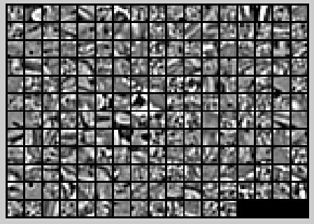
patches = sampleIMAGES;
display_network(patches(:,randi(size(patches,2),200,1)),8);
% Obtain random parameters theta
theta = initializeParameters(hiddenSize, visibleSize);
%%======================================================================
%% STEP 2: Implement sparseAutoencoderCost
%
% You can implement all of the components (squared error cost, weight decay term,
% sparsity penalty) in the cost function at once, but it may be easier to do
% it step-by-step and run gradient checking (see STEP 3) after each step. We
% suggest implementing the sparseAutoencoderCost function using the following steps:
%
% (a) Implement forward propagation in your neural network, and implement the
% squared error term of the cost function. Implement backpropagation to
% compute the derivatives. Then (using lambda=beta=0), run Gradient Checking
% to verify that the calculations corresponding to the squared error cost
% term are correct.
%
% (b) Add in the weight decay term (in both the cost function and the derivative
% calculations), then re-run Gradient Checking to verify correctness.
%
% (c) Add in the sparsity penalty term, then re-run Gradient Checking to
% verify correctness.
%
% Feel free to change the training settings when debugging your
% code. (For example, reducing the training set size or
% number of hidden units may make your code run faster; and setting beta
% and/or lambda to zero may be helpful for debugging.) However, in your
% final submission of the visualized weights, please use parameters we
% gave in Step 0 above.
[cost, grad] = sparseAutoencoderCost(theta, visibleSize, hiddenSize, lambda, ...
sparsityParam, beta, patches);
%%======================================================================
%% STEP 3: Gradient Checking
%
% Hint: If you are debugging your code, performing gradient checking on smaller models
% and smaller training sets (e.g., using only 10 training examples and 1-2 hidden
% units) may speed things up.
% First, lets make sure your numerical gradient computation is correct for a
% simple function. After you have implemented computeNumericalGradient.m,
% run the following:
checkNumericalGradient();
% Now we can use it to check your cost function and derivative calculations
% for the sparse autoencoder.
numgrad = computeNumericalGradient( @(x) sparseAutoencoderCost(x, visibleSize, ...
hiddenSize, lambda,sparsityParam,...
beta,patches), theta);
% Use this to visually compare the gradients side by side
disp([numgrad grad]);
% Compare numerically computed gradients with the ones obtained from backpropagation
diff = norm(numgrad-grad)/norm(numgrad+grad);
disp(diff); % Should be small. In our implementation, these values are
% usually less than 1e-9.
% When you got this working, Congratulations!!!
%%======================================================================
%% STEP 4: After verifying that your implementation of
% sparseAutoencoderCost is correct, You can start training your sparse
% autoencoder with minFunc (L-BFGS).
% Randomly initialize the parameters
theta = initializeParameters(hiddenSize, visibleSize);
% Use minFunc to minimize the function
addpath minFunc/
options.Method = 'lbfgs'; % Here, we use L-BFGS to optimize our cost
% function. Generally, for minFunc to work, you
% need a function pointer with two outputs: the
% function value and the gradient. In our problem,
% sparseAutoencoderCost.m satisfies this.
options.maxIter = 400; % Maximum number of iterations of L-BFGS to run
options.display = 'on';
[opttheta, cost] = minFunc( @(p) sparseAutoencoderCost(p, ...
visibleSize, hiddenSize, ...
lambda, sparsityParam, ...
beta, patches), ...
theta, options);
%%======================================================================
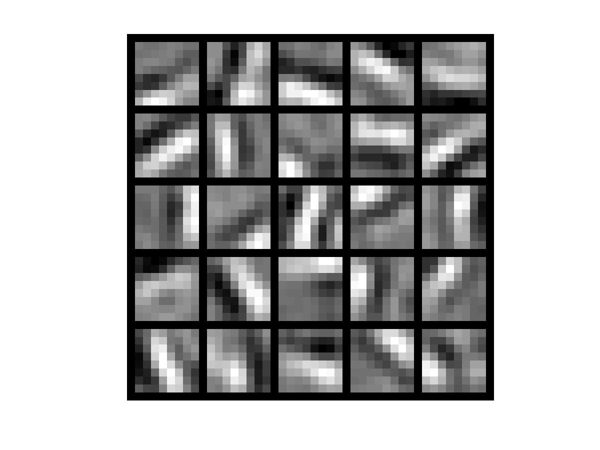
%% STEP 5: Visualization
W1 = reshape(opttheta(1:hiddenSize*visibleSize), hiddenSize, visibleSize);
display_network(W1', 12);
print -djpeg weights.jpg % save the visualization to a file
sampleIMAGES.m,进行图像采集
function patches = sampleIMAGES()
% sampleIMAGES
% Returns 10000 patches for training

load IMAGES;    % load images from disk
% figure;
% imagesc(IMAGES(:,:,6));
% colormap gray;
patchsize = 8;  % we'll use 8x8 patches
numpatches = 10000;

% Initialize patches with zeros.  Your code will fill in this matrix--one
% column per patch, 10000 columns.
patches = zeros(patchsize*patchsize, numpatches);

%% ---------- YOUR CODE HERE --------------------------------------
%  Instructions: Fill in the variable called "patches" using data
%  from IMAGES.
%
%  IMAGES is a 3D array containing 10 images
%  For instance, IMAGES(:,:,6) is a 512x512 array containing the 6th image,
%  and you can type "imagesc(IMAGES(:,:,6)), colormap gray;" to visualize
%  it. (The contrast on these images look a bit off because they have
%  been preprocessed using using "whitening."  See the lecture notes for
%  more details.) As a second example, IMAGES(21:30,21:30,1) is an image
%  patch corresponding to the pixels in the block (21,21) to (30,30) of
%  Image 1
[m,n] = size(IMAGES(:,:,1));
for i = 1:10
    image = IMAGES(:, :, i);
    for j = 1:1000
        row_id     = randi([1 (m - patchsize + 1)]);
        column_id  = randi([1 (n - patchsize + 1)]);
        patches(:,(i-1)*1000+j) = reshape(image(row_id:(row_id+patchsize-1), column_id:(column_id+patchsize-1)),...
            patchsize*patchsize, 1);
    end
end
%% ---------------------------------------------------------------
% For the autoencoder to work well we need to normalize the data
% Specifically, since the output of the network is bounded between [0,1]
% (due to the sigmoid activation function), we have to make sure
% the range of pixel values is also bounded between [0,1]
patches = normalizeData(patches);

end


%% ---------------------------------------------------------------
function patches = normalizeData(patches)

% Squash data to [0.1, 0.9] since we use sigmoid as the activation
% function in the output layer

% Remove DC (mean of images).
patches = bsxfun(@minus, patches, mean(patches));

% Truncate to +/-3 standard deviations and scale to -1 to 1
pstd = 3 * std(patches(:));
patches = max(min(patches, pstd), -pstd) / pstd;

% Rescale from [-1,1] to [0.1,0.9]
patches = (patches + 1) * 0.4 + 0.1;

end
function [cost,grad] = sparseAutoencoderCost(theta, visibleSize, hiddenSize, ...
                                             lambda, sparsityParam, beta, data)

% visibleSize: the number of input units (probably 64)
% hiddenSize: the number of hidden units (probably 25)
% lambda: weight decay parameter
% sparsityParam: The desired average activation for the hidden units (denoted in the lecture
%                           notes by the greek alphabet rho, which looks like a lower-case "p").
% beta: weight of sparsity penalty term
% data: Our 64x10000 matrix containing the training data.  So, data(:,i) is the i-th training example.

% The input theta is a vector (because minFunc expects the parameters to be a vector).
% We first convert theta to the (W1, W2, b1, b2) matrix/vector format, so that this
% follows the notation convention of the lecture notes.

W1 = reshape(theta(1:hiddenSize*visibleSize), hiddenSize, visibleSize);
W2 = reshape(theta(hiddenSize*visibleSize+1:2*hiddenSize*visibleSize), visibleSize, hiddenSize);
b1 = theta(2*hiddenSize*visibleSize+1:2*hiddenSize*visibleSize+hiddenSize);
b2 = theta(2*hiddenSize*visibleSize+hiddenSize+1:end);

% Cost and gradient variables (your code needs to compute these values).
% Here, we initialize them to zeros.
cost = 0;
W1grad = zeros(size(W1));
W2grad = zeros(size(W2));
b1grad = zeros(size(b1));
b2grad = zeros(size(b2));

%% ---------- YOUR CODE HERE --------------------------------------
%  Instructions: Compute the cost/optimization objective J_sparse(W,b) for the Sparse Autoencoder,
%                and the corresponding gradients W1grad, W2grad, b1grad, b2grad.
%
% W1grad, W2grad, b1grad and b2grad should be computed using backpropagation.
% Note that W1grad has the same dimensions as W1, b1grad has the same dimensions
% as b1, etc.  Your code should set W1grad to be the partial derivative of J_sparse(W,b) with
% respect to W1.  I.e., W1grad(i,j) should be the partial derivative of J_sparse(W,b)
% with respect to the input parameter W1(i,j).  Thus, W1grad should be equal to the term
% [(1/m) Delta W^{(1)} + lambda W^{(1)}] in the last block of pseudo-code in Section 2.2
% of the lecture notes (and similarly for W2grad, b1grad, b2grad).
%
% Stated differently, if we were using batch gradient descent to optimize the parameters,
% the gradient descent update to W1 would be W1 := W1 - alpha * W1grad, and similarly for W2, b1, b2.
%
Jcost = 0;   % 预测误差项
Jweight = 0; % 权重衰减项
Jsparse = 0; % 稀疏惩罚项
[n,m] = size(data); %m是样本个数,n是样本特征数

%前向传播计算神经网络每个神经元的激活值
Z2 = W1 * data + repmat(b1, 1, m); %b1扩展成1行m列,因为对每个样本的每个隐单元的激活值都要加上偏置项
a2 = sigmoid(Z2);
Z3 = W2 * a2 + repmat(b2, 1, m);
a3 = sigmoid(Z3);

%计算预测产生的误差项
Jcost = (0.5 / m) * sum(sum((a3 - data).^2));

%计算权重衰减项
Jweight = 0.5 * (sum(sum(W1.^2)) + sum(sum(W2.^2)));

%计算稀疏惩罚项
rho = (1 / m) .* sum(a2, 2);
Jsparse = sum(sparsityParam .* log(sparsityParam ./ rho) + ...
        (1- sparsityParam) .* log((1- sparsityParam) ./ (1 - rho)));
%代价函数
cost = Jcost + lambda * Jweight + beta * Jsparse;

%反向传播求出每个节点的误差
d3 = -(data - a3) .* (sigmoid(Z3) .* (1 - sigmoid(Z3)));%注意sigmoid函数的求导f(1-f)
sparseterm = beta * (-sparsityParam ./ rho + ...
            (1- sparsityParam) ./ (1 - rho)); %稀疏项导数
d2 = (W2' * d3 + repmat(sparseterm,1,m)).*(sigmoid(Z2) .* (1 - sigmoid(Z2)));

%计算W1grad
W1grad = W1grad + d2 * data';
W1grad = (1/m) * W1grad + lambda * W1;

%计算W2grad
W2grad = W2grad+d3*a2';
W2grad = (1/m) * W2grad + lambda * W2;

%计算b1grad
b1grad = b1grad+sum(d2,2);
b1grad = (1/m)*b1grad;%注意b的偏导是一个向量,所以这里应该把每一行的值累加起来

%计算b2grad
b2grad = b2grad+sum(d3,2);
b2grad = (1/m)*b2grad;

%-------------------------------------------------------------------
% After computing the cost and gradient, we will convert the gradients back
% to a vector format (suitable for minFunc).  Specifically, we will unroll
% your gradient matrices into a vector.

grad = [W1grad(:) ; W2grad(:) ; b1grad(:) ; b2grad(:)];

end

%-------------------------------------------------------------------
% Here's an implementation of the sigmoid function, which you may find useful
% in your computation of the costs and the gradients.  This inputs a (row or
% column) vector (say (z1, z2, z3)) and returns (f(z1), f(z2), f(z3)).

function sigm = sigmoid(x)

    sigm = 1 ./ (1 + exp(-x));
end
function numgrad = computeNumericalGradient(J, theta)
% numgrad = computeNumericalGradient(J, theta)
% theta: a vector of parameters
% J: a function that outputs a real-number. Calling y = J(theta) will return the
% function value at theta.

% Initialize numgrad with zeros
numgrad = zeros(size(theta));

%% ---------- YOUR CODE HERE --------------------------------------
% Instructions:
% Implement numerical gradient checking, and return the result in numgrad.
% (See Section 2.3 of the lecture notes.)
% You should write code so that numgrad(i) is (the numerical approximation to) the
% partial derivative of J with respect to the i-th input argument, evaluated at theta.
% I.e., numgrad(i) should be the (approximately) the partial derivative of J with
% respect to theta(i).
%
% Hint: You will probably want to compute the elements of numgrad one at a time.
epsilon = 1e-4;
n = size(theta,1);
E = eye(n);
for i = 1:n
    delta = E(:,i)*epsilon;
    numgrad(i) = (J(theta+delta)-J(theta-delta))/(epsilon*2.0);
end


%% ---------------------------------------------------------------
end
function [] = checkNumericalGradient()
% This code can be used to check your numerical gradient implementation
% in computeNumericalGradient.m
% It analytically evaluates the gradient of a very simple function called
% simpleQuadraticFunction (see below) and compares the result with your numerical
% solution. Your numerical gradient implementation is incorrect if
% your numerical solution deviates too much from the analytical solution.

% Evaluate the function and gradient at x = [4; 10]; (Here, x is a 2d vector.)
x = [4; 10];
[value, grad] = simpleQuadraticFunction(x);

% Use your code to numerically compute the gradient of simpleQuadraticFunction at x.
% (The notation "@simpleQuadraticFunction" denotes a pointer to a function.)
numgrad = computeNumericalGradient(@simpleQuadraticFunction, x);

% Visually examine the two gradient computations.  The two columns
% you get should be very similar.
disp([numgrad grad]);
fprintf('The above two columns you get should be very similar.
(Left-Your Numerical Gradient, Right-Analytical Gradient)

');

% Evaluate the norm of the difference between two solutions.
% If you have a correct implementation, and assuming you used EPSILON = 0.0001
% in computeNumericalGradient.m, then diff below should be 2.1452e-12
diff = norm(numgrad-grad)/norm(numgrad+grad);
disp(diff);
fprintf('Norm of the difference between numerical and analytical gradient (should be < 1e-9)

');
end


function [value,grad] = simpleQuadraticFunction(x)
% this function accepts a 2D vector as input.
% Its outputs are:
%   value: h(x1, x2) = x1^2 + 3*x1*x2
%   grad: A 2x1 vector that gives the partial derivatives of h with respect to x1 and x2
% Note that when we pass @simpleQuadraticFunction(x) to computeNumericalGradients, we're assuming
% that computeNumericalGradients will use only the first returned value of this function.

value = x(1)^2 + 3*x(1)*x(2);

grad = zeros(2, 1);
grad(1)  = 2*x(1) + 3*x(2);
grad(2)  = 3*x(1);

end
function [h, array] = display_network(A, opt_normalize, opt_graycolor, cols, opt_colmajor)
% This function visualizes filters in matrix A. Each column of A is a
% filter. We will reshape each column into a square image and visualizes
% on each cell of the visualization panel.
% All other parameters are optional, usually you do not need to worry
% about it.
% opt_normalize: whether we need to normalize the filter so that all of
% them can have similar contrast. Default value is true.
% opt_graycolor: whether we use gray as the heat map. Default is true.
% cols: how many columns are there in the display. Default value is the
% squareroot of the number of columns in A.
% opt_colmajor: you can switch convention to row major for A. In that
% case, each row of A is a filter. Default value is false.
warning off all

if ~exist('opt_normalize', 'var') || isempty(opt_normalize)
    opt_normalize= true;
end

if ~exist('opt_graycolor', 'var') || isempty(opt_graycolor)
    opt_graycolor= true;
end

if ~exist('opt_colmajor', 'var') || isempty(opt_colmajor)
    opt_colmajor = false;
end

% rescale
A = A - mean(A(:));

if opt_graycolor, colormap(gray); end

% compute rows, cols
[L M]=size(A);
sz=sqrt(L);
buf=1;
if ~exist('cols', 'var')
    if floor(sqrt(M))^2 ~= M
        n=ceil(sqrt(M));
        while mod(M, n)~=0 && n<1.2*sqrt(M), n=n+1; end
        m=ceil(M/n);
    else
        n=sqrt(M);
        m=n;
    end
else
    n = cols;
    m = ceil(M/n);
end

array=-ones(buf+m*(sz+buf),buf+n*(sz+buf));

if ~opt_graycolor
    array = 0.1.* array;
end


if ~opt_colmajor
    k=1;
    for i=1:m
        for j=1:n
            if k>M,
                continue;
            end
            clim=max(abs(A(:,k)));
            if opt_normalize
                array(buf+(i-1)*(sz+buf)+(1:sz),buf+(j-1)*(sz+buf)+(1:sz))=reshape(A(:,k),sz,sz)/clim;
            else
                array(buf+(i-1)*(sz+buf)+(1:sz),buf+(j-1)*(sz+buf)+(1:sz))=reshape(A(:,k),sz,sz)/max(abs(A(:)));
            end
            k=k+1;
        end
    end
else
    k=1;
    for j=1:n
        for i=1:m
            if k>M,
                continue;
            end
            clim=max(abs(A(:,k)));
            if opt_normalize
                array(buf+(i-1)*(sz+buf)+(1:sz),buf+(j-1)*(sz+buf)+(1:sz))=reshape(A(:,k),sz,sz)/clim;
            else
                array(buf+(i-1)*(sz+buf)+(1:sz),buf+(j-1)*(sz+buf)+(1:sz))=reshape(A(:,k),sz,sz);
            end
            k=k+1;
        end
    end
end

if opt_graycolor
    h=imagesc(array,'EraseMode','none',[-1 1]);
else
    h=imagesc(array,'EraseMode','none',[-1 1]);
end
axis image off

drawnow;

warning on all
进行梯度检验,两种不同的方式计算出的梯度相差 7.2299e-11,远小于1e-9.
随机展示出所有采样图像中的200幅:
本程序主要耗时间的地方是梯度检验,大约4-5分钟.
最终学习出的权重可视化结果如下: