建立一个逻辑回归模型来预测一个学生是否被录取。
![]()
import numpy as np
import pandas as pd
import matplotlib.pyplot as plt
import os
path='data'+os.sep+'Logireg_data.txt'
pdData=pd.read_csv(path,header=None,names=['Exam1','Exam2','Admitted'])
pdData.head()
print(pdData.head())
print(pdData.shape)
positive=pdData[pdData['Admitted']==1]#定义正
nagative=pdData[pdData['Admitted']==0]#定义负
fig,ax=plt.subplots(figsize=(10,5))
ax.scatter(positive['Exam1'],positive['Exam2'],s=30,c='b',marker='o',label='Admitted')
ax.scatter(nagative['Exam1'],nagative['Exam2'],s=30,c='r',marker='x',label='not Admitted')
ax.legend()
ax.set_xlabel('Exam 1 score')
ax.set_ylabel('Exam 2 score')
plt.show()#画图
##实现算法 the logistics regression 目标建立一个分类器 设置阈值来判断录取结果
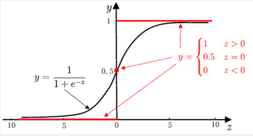
##sigmoid 函数
def sigmoid(z):
return 1/(1+np.exp(-z))
#画图
nums=np.arange(-10,10,step=1)
fig,ax=plt.subplots(figsize=(12,4))
ax.plot(nums,sigmoid(nums),'r')#画图定义
plt.show()
#按照理论实现预测函数
def model(X,theta):
return sigmoid(np.dot(X,theta.T))
pdData.insert(0,'ones',1)#插入一列
orig_data=pdData.as_matrix()
cols=orig_data.shape[1]
X=orig_data[:,0:cols-1]
y=orig_data[:,cols-1:cols]
theta=np.zeros([1,3])
print(X[:5])
print(X.shape,y.shape,theta.shape)
##损失函数
def cost(X,y,theta):
left=np.multiply(-y,np.log(model(X,theta)))
right=np.multiply(1-y,np.log(1-model(X,theta)))
return np.sum(left-right)/(len(X))
print(cost(X,y,theta))
#计算梯度
def gradient(X, y, theta):
grad = np.zeros(theta.shape)
error = (model(X, theta) - y).ravel()
for j in range(len(theta.ravel())): # for each parmeter
term = np.multiply(error, X[:, j])
grad[0, j] = np.sum(term) / len(X)
return grad
##比较3种不同梯度下降方法
STOP_ITER=0
STOP_COST=1
STOP_GRAD=2
def stopCriterion(type,value,threshold):
if type==STOP_ITER: return value>threshold
elif type==STOP_COST: return abs(value[-1]-value[-2])<threshold
elif type==STOP_GRAD: return np.linalg.norm(value)<threshold
import numpy.random
#打乱数据洗牌
def shuffledata(data):
np.random.shuffle(data)
cols=data.shape[1]
X=data[:,0:cols-1]
y=data[:,cols-1:]
return X,y
import time
def descent(data, theta, batchSize, stopType, thresh, alpha):
# 梯度下降求解
init_time = time.time()
i = 0 # 迭代次数
k = 0 # batch
X, y = shuffledata(data)
grad = np.zeros(theta.shape) # 计算的梯度
costs = [cost(X, y, theta)] # 损失值
while True:
grad = gradient(X[k:k + batchSize], y[k:k + batchSize], theta)
k += batchSize # 取batch数量个数据
if k >= n:
k = 0
X, y = shuffledata(data) # 重新洗牌
theta = theta - alpha * grad # 参数更新
costs.append(cost(X, y, theta)) # 计算新的损失
i += 1
if stopType == STOP_ITER:
value = i
elif stopType == STOP_COST:
value = costs
elif stopType == STOP_GRAD:
value = grad
if stopCriterion(stopType, value, thresh): break
return theta, i - 1, costs, grad, time.time() - init_time
#选择梯度下降
def runExpe(data, theta, batchSize, stopType, thresh, alpha):
#import pdb; pdb.set_trace();
theta, iter, costs, grad, dur = descent(data, theta, batchSize, stopType, thresh, alpha)
name = "Original" if (data[:,1]>2).sum() > 1 else "Scaled"
name += " data - learning rate: {} - ".format(alpha)
if batchSize==n: strDescType = "Gradient"
elif batchSize==1: strDescType = "Stochastic"
else: strDescType = "Mini-batch ({})".format(batchSize)
name += strDescType + " descent - Stop: "
if stopType == STOP_ITER: strStop = "{} iterations".format(thresh)
elif stopType == STOP_COST: strStop = "costs change < {}".format(thresh)
else: strStop = "gradient norm < {}".format(thresh)
name += strStop
print ("***{}
Theta: {} - Iter: {} - Last cost: {:03.2f} - Duration: {:03.2f}s".format(
name, theta, iter, costs[-1], dur))
fig, ax = plt.subplots(figsize=(12,4))
ax.plot(np.arange(len(costs)), costs, 'r')
ax.set_xlabel('Iterations')
ax.set_ylabel('Cost')
ax.set_title(name.upper() + ' - Error vs. Iteration')
return theta
n= 100
runExpe(orig_data,theta,n,STOP_ITER,thresh=5000,alpha=0.000001)
plt.show()
runExpe(orig_data,theta,n,STOP_GRAD,thresh=0.05,alpha=0.001)
plt.show()
runExpe(orig_data,theta,n,STOP_COST,thresh=0.000001,alpha=0.001)
plt.show()
#对比
runExpe(orig_data, theta, 1, STOP_ITER, thresh=5000, alpha=0.001)
plt.show()
runExpe(orig_data, theta, 1, STOP_ITER, thresh=15000, alpha=0.000002)
plt.show()
runExpe(orig_data, theta, 16, STOP_ITER, thresh=15000, alpha=0.001)
plt.show()
##对数据进行标准化 将数据按其属性(按列进行)减去其均值,然后除以其方差。
#最后得到的结果是,对每个属性/每列来说所有数据都聚集在0附近,方差值为1
from sklearn import preprocessing as pp
scaled_data = orig_data.copy()
scaled_data[:, 1:3] = pp.scale(orig_data[:, 1:3])
runExpe(scaled_data, theta, n, STOP_ITER, thresh=5000, alpha=0.001)
#设定阈值
def predict(X, theta):
return [1 if x >= 0.5 else 0 for x in model(X, theta)]
# if __name__=='__main__':
scaled_X = scaled_data[:, :3]
y = scaled_data[:, 3]
predictions = predict(scaled_X, theta)
correct = [1 if ((a == 1 and b == 1) or (a == 0 and b == 0)) else 0 for (a, b) in zip(predictions, y)]
accuracy = (sum(map(int, correct)) % len(correct))
print ('accuracy = {0}%'.format(accuracy))
运行结果
    Exam1      Exam2  Admitted
0  34.623660  78.024693         0
1  30.286711  43.894998         0
2  35.847409  72.902198         0
3  60.182599  86.308552         1
4  79.032736  75.344376         1
(100, 3)
[[ 1.         34.62365962 78.02469282]
 [ 1.         30.28671077 43.89499752]
 [ 1.         35.84740877 72.90219803]
 [ 1.         60.18259939 86.3085521 ]
 [ 1.         79.03273605 75.34437644]]
(100, 3) (100, 1) (1, 3)
0.6931471805599453
***Original data - learning rate: 1e-06 - Gradient descent - Stop: 5000 iterations
Theta: [[-0.00027127  0.00705232  0.00376711]] - Iter: 5000 - Last cost: 0.63 - Duration: 1.42s
***Original data - learning rate: 0.001 - Gradient descent - Stop: gradient norm < 0.05
Theta: [[-2.37033409  0.02721692  0.01899456]] - Iter: 40045 - Last cost: 0.49 - Duration: 11.63s
***Original data - learning rate: 0.001 - Gradient descent - Stop: costs change < 1e-06
Theta: [[-5.13364014  0.04771429  0.04072397]] - Iter: 109901 - Last cost: 0.38 - Duration: 32.27s
***Original data - learning rate: 0.001 - Stochastic descent - Stop: 5000 iterations
Theta: [[-0.36946801  0.0618896   0.05188799]] - Iter: 5000 - Last cost: 2.28 - Duration: 0.60s
***Original data - learning rate: 2e-06 - Stochastic descent - Stop: 15000 iterations
Theta: [[-0.00201976  0.01010609  0.00105193]] - Iter: 15000 - Last cost: 0.63 - Duration: 1.67s
***Original data - learning rate: 0.001 - Mini-batch (16) descent - Stop: 15000 iterations
Theta: [[-1.03184406  0.02958433  0.02230517]] - Iter: 15000 - Last cost: 0.80 - Duration: 2.10s
***Scaled data - learning rate: 0.001 - Gradient descent - Stop: 5000 iterations
Theta: [[0.3080807  0.86494967 0.77367651]] - Iter: 5000 - Last cost: 0.38 - Duration: 1.51s
accuracy = 60%
程序用到的测试数据:
链接:https://pan.baidu.com/s/1Enr4JcPVzBiUCfvEYiVmlQ
提取码:lg51