CS190.1x-ML_lab5_pca_student

这次lab也是最后一次lab了，前面两次lab介绍了回归和分类，特别详细地介绍了线性回归和逻辑回归，这次的作业主要是非监督学习——降维，主要是PCA。数据集是神经科学的数据，来自于Ahrens Lab，数据公布在CodeNeuro data repository。相关ipynb文件见我github。

这次的数据主要是研究幼年斑马鱼的运动产生的。由于斑马鱼是透明的，所以神经科学经常拿它来做研究，观察整个大脑的活动。本次的数据集是随着时间变化的、包含斑马鱼大脑神经活动的图像。

这次Lab包含四个部分：样本集上用PCA；实现PCA函数和评价PCA效果；把PCA用于本次数据集；用PCA来实现基于特征的聚集。

Part 1 Work through the steps of PCA on a sample dataset

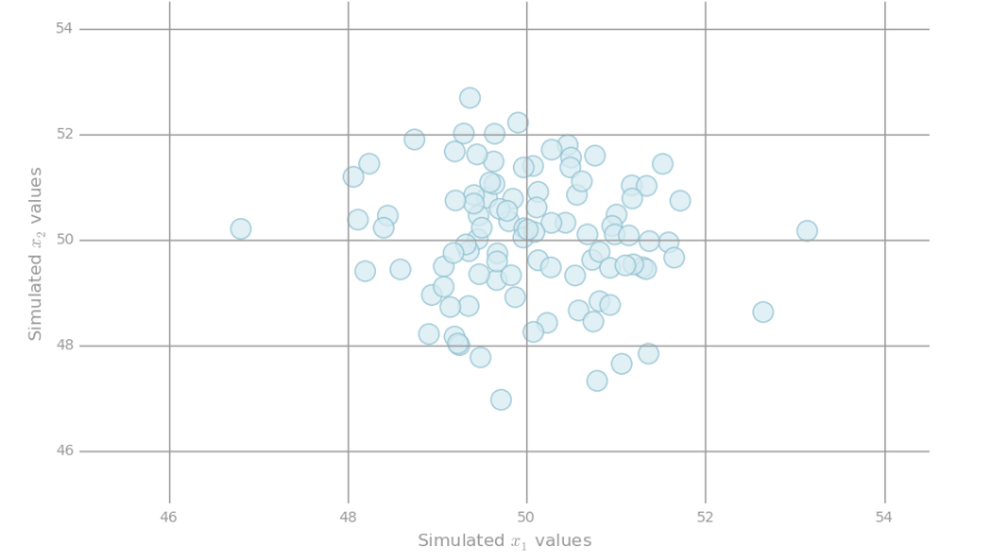
PCA是降维的常用方法，为了理解PCA，我们这里自己构造满足2维的高斯分布的数据，其中，均值是50，方差是1。为了理解PCA，我们这里用两个协方差：0和0.9。下面我们画出两个图。

import matplotlib.pyplot as plt
import numpy as np

def preparePlot(xticks, yticks, figsize=(10.5, 6), hideLabels=False, gridColor='#999999',
                gridWidth=1.0):
    """Template for generating the plot layout."""
    plt.close()
    fig, ax = plt.subplots(figsize=figsize, facecolor='white', edgecolor='white')
    ax.axes.tick_params(labelcolor='#999999', labelsize='10')
    for axis, ticks in [(ax.get_xaxis(), xticks), (ax.get_yaxis(), yticks)]:
        axis.set_ticks_position('none')
        axis.set_ticks(ticks)
        axis.label.set_color('#999999')
        if hideLabels: axis.set_ticklabels([])
    plt.grid(color=gridColor, linewidth=gridWidth, linestyle='-')
    map(lambda position: ax.spines[position].set_visible(False), ['bottom', 'top', 'left', 'right'])
    return fig, ax

def create2DGaussian(mn, sigma, cov, n):
    """Randomly sample points from a two-dimensional Gaussian distribution"""
    np.random.seed(142)
    return np.random.multivariate_normal(np.array([mn, mn]), np.array([[sigma, cov], [cov, sigma]]), n)

dataRandom = create2DGaussian(mn=50, sigma=1, cov=0, n=100)

# generate layout and plot data
fig, ax = preparePlot(np.arange(46, 55, 2), np.arange(46, 55, 2))
ax.set_xlabel(r'Simulated $x_1$ values'), ax.set_ylabel(r'Simulated $x_2$ values')
ax.set_xlim(45, 54.5), ax.set_ylim(45, 54.5)
plt.scatter(dataRandom[:,0], dataRandom[:,1], s=14**2, c='#d6ebf2', edgecolors='#8cbfd0', alpha=0.75)
pass

dataCorrelated = create2DGaussian(mn=50, sigma=1, cov=.9, n=100)

# generate layout and plot data
fig, ax = preparePlot(np.arange(46, 55, 2), np.arange(46, 55, 2))
ax.set_xlabel(r'Simulated $x_1$ values'), ax.set_ylabel(r'Simulated $x_2$ values')
ax.set_xlim(45.5, 54.5), ax.set_ylim(45.5, 54.5)
plt.scatter(dataCorrelated[:,0], dataCorrelated[:,1], s=14**2, c='#d6ebf2',
            edgecolors='#8cbfd0', alpha=0.75)
pass

Interpreting PCA

PCA可以解释为数据变化最大的方向。实现PCA的第一步是找到数据的中心点：计算每个特征的平均值，然后每个特征减去其对应的平均值。

# TODO: Replace <FILL IN> with appropriate code
correlatedData = sc.parallelize(dataCorrelated)

meanCorrelated = correlatedData.mean()
correlatedDataZeroMean = correlatedData.map(lambda x:x-meanCorrelated)

print meanCorrelated
print correlatedData.take(1)
print correlatedDataZeroMean.take(1)

Sample covariance matrix

在上面的基础上，计算协方差矩阵。主要思路是利用np.outer()来计算，这个思路之前就碰到过。

# TODO: Replace <FILL IN> with appropriate code
# Compute the covariance matrix using outer products and correlatedDataZeroMean
correlatedCov = correlatedDataZeroMean.map(lambda x: np.outer(x,x)).sum()/correlatedDataZeroMean.count()
print correlatedCov

Covariance Function

把上面的全部综合起来

# TODO: Replace <FILL IN> with appropriate code
def estimateCovariance(data):
    """Compute the covariance matrix for a given rdd.

    Note:
        The multi-dimensional covariance array should be calculated using outer products.  Don't
        forget to normalize the data by first subtracting the mean.

    Args:
        data (RDD of np.ndarray):  An `RDD` consisting of NumPy arrays.

    Returns:
        np.ndarray: A multi-dimensional array where the number of rows and columns both equal the
            length of the arrays in the input `RDD`.
    """
    means = data.sum()/float(data.count())
    return data.map(lambda x:x-means).map(lambda x:np.outer(x,x)).sum()/float(data.count())

correlatedCovAuto= estimateCovariance(correlatedData)
print correlatedCovAuto

Eigendecomposition

我们在计算协方差矩阵后，下面进行特征分解，找到特征值和特征向量。其中特征向量就是我们要找的最大方差的方向，也叫“主成份”（principle components），特征值就是这个方向上的方差。

计算dd的协方差矩阵的时间复杂度是 O(dd*d）。不过一般来说d都比较小，可以本地计算。我们一般用numpy.linalg里的eigh()方法来计算。

# TODO: Replace <FILL IN> with appropriate code
from numpy.linalg import eigh

# Calculate the eigenvalues and eigenvectors from correlatedCovAuto
eigVals, eigVecs =eigh(correlatedCovAuto)
print 'eigenvalues: {0}'.format(eigVals)
print '
eigenvectors: 
{0}'.format(eigVecs)

# Use np.argsort to find the top eigenvector based on the largest eigenvalue
inds = np.argsort(eigVals)[::-1]
topComponent = eigVecs[:,inds[0]]
print '
top principal component: {0}'.format(topComponent)

PCA scores

通过上面的步骤，我们可以得到principle component。然后把数据中的元素和这个相乘，即12的矩阵乘以21的矩阵，得到一个数，从而把原来的矩阵从2维降到了1维。

# TODO: Replace <FILL IN> with appropriate code
# Use the topComponent and the data from correlatedData to generate PCA scores
correlatedDataScores = correlatedData.map(lambda x:np.dot(x,topComponent))
print 'one-dimensional data (first three):
{0}'.format(np.asarray(correlatedDataScores.take(3)))

Part 2 Write a PCA function and evaluate PCA on sample datasets

PCA function

通过上面的学习，我们这里直接实现pca的函数。

# TODO: Replace <FILL IN> with appropriate code
def pca(data, k=2):
    """Computes the top `k` principal components, corresponding scores, and all eigenvalues.

    Note:
        All eigenvalues should be returned in sorted order (largest to smallest). `eigh` returns
        each eigenvectors as a column.  This function should also return eigenvectors as columns.

    Args:
        data (RDD of np.ndarray): An `RDD` consisting of NumPy arrays.
        k (int): The number of principal components to return.

    Returns:
        tuple of (np.ndarray, RDD of np.ndarray, np.ndarray): A tuple of (eigenvectors, `RDD` of
            scores, eigenvalues).  Eigenvectors is a multi-dimensional array where the number of
            rows equals the length of the arrays in the input `RDD` and the number of columns equals
            `k`.  The `RDD` of scores has the same number of rows as `data` and consists of arrays
            of length `k`.  Eigenvalues is an array of length d (the number of features).
    """
    dataCov = estimateCovariance(data)
    eigVals, eigVecs = eigh(dataCov)
    inds = np.argsort(eigVals)[::-1]
    # Return the `k` principal components, `k` scores, and all eigenvalues
    return (eigVecs[:,inds[:k]],data.map(lambda x:np.dot(x,eigVecs[:,inds[:k]])),eigVals[inds])

# Run pca on correlatedData with k = 2
topComponentsCorrelated, correlatedDataScoresAuto, eigenvaluesCorrelated = pca(correlatedData,2)

# Note that the 1st principal component is in the first column
print 'topComponentsCorrelated: 
{0}'.format(topComponentsCorrelated)
print ('
correlatedDataScoresAuto (first three): 
{0}'
       .format('
'.join(map(str, correlatedDataScoresAuto.take(3)))))
print '
eigenvaluesCorrelated: 
{0}'.format(eigenvaluesCorrelated)

# Create a higher dimensional test set
pcaTestData = sc.parallelize([np.arange(x, x + 4) for x in np.arange(0, 20, 4)])
componentsTest, testScores, eigenvaluesTest = pca(pcaTestData, 3)

print '
pcaTestData: 
{0}'.format(np.array(pcaTestData.collect()))
print '
componentsTest: 
{0}'.format(componentsTest)
print ('
testScores (first three): 
{0}'
       .format('
'.join(map(str, testScores.take(3)))))
print '
eigenvaluesTest: 
{0}'.format(eigenvaluesTest)

PCA on dataRandom

# TODO: Replace <FILL IN> with appropriate code
randomData = sc.parallelize(dataRandom)

# Use pca on randomData
topComponentsRandom, randomDataScoresAuto, eigenvaluesRandom = pca(randomData,2)

print 'topComponentsRandom: 
{0}'.format(topComponentsRandom)
print ('
randomDataScoresAuto (first three): 
{0}'
       .format('
'.join(map(str, randomDataScoresAuto.take(3)))))
print '
eigenvaluesRandom: 
{0}'.format(eigenvaluesRandom)

3D to 2D

# TODO: Replace <FILL IN> with appropriate code
threeDData = sc.parallelize(dataThreeD)
componentsThreeD, threeDScores, eigenvaluesThreeD = pca(threeDData,2)

print 'componentsThreeD: 
{0}'.format(componentsThreeD)
print ('
threeDScores (first three): 
{0}'
       .format('
'.join(map(str, threeDScores.take(3)))))
print '
eigenvaluesThreeD: 
{0}'.format(eigenvaluesThreeD)

Variance explained

计算我们选择的前K个方差的和占总的方差的比例

# TODO: Replace <FILL IN> with appropriate code
def varianceExplained(data, k=1):
    """Calculate the fraction of variance explained by the top `k` eigenvectors.

    Args:
        data (RDD of np.ndarray): An RDD that contains NumPy arrays which store the
            features for an observation.
        k: The number of principal components to consider.

    Returns:
        float: A number between 0 and 1 representing the percentage of variance explained
            by the top `k` eigenvectors.
    """
    components, scores, eigenvalues = pca(data,k)
    return np.sum(eigenvalues[:k])/float(np.sum(eigenvalues))

varianceRandom1 = varianceExplained(randomData, 1)
varianceCorrelated1 = varianceExplained(correlatedData, 1)
varianceRandom2 = varianceExplained(randomData, 2)
varianceCorrelated2 = varianceExplained(correlatedData, 2)
varianceThreeD2 = varianceExplained(threeDData, 2)
print ('Percentage of variance explained by the first component of randomData: {0:.1f}%'
       .format(varianceRandom1 * 100))
print ('Percentage of variance explained by both components of randomData: {0:.1f}%'
       .format(varianceRandom2 * 100))
print ('
Percentage of variance explained by the first component of correlatedData: {0:.1f}%'.
       format(varianceCorrelated1 * 100))
print ('Percentage of variance explained by both components of correlatedData: {0:.1f}%'
       .format(varianceCorrelated2 * 100))
print ('
Percentage of variance explained by the first two components of threeDData: {0:.1f}%'
       .format(varianceThreeD2 * 100))

Part 3 Parse, inspect, and preprocess neuroscience data then perform PCA

Load neuroscience data

这一部分将用到真实的数据，第一步当然是预处理数据。

import os
baseDir = os.path.join('data')
inputPath = os.path.join('cs190', 'neuro.txt')

inputFile = os.path.join(baseDir, inputPath)

lines = sc.textFile(inputFile)
print lines.first()[0:100]

# Check that everything loaded properly
assert len(lines.first()) == 1397
assert lines.count() == 46460

Parse the data

# TODO: Replace <FILL IN> with appropriate code
def parse(line):
    """Parse the raw data into a (`tuple`, `np.ndarray`) pair.

    Note:
        You should store the pixel coordinates as a tuple of two ints and the elements of the pixel intensity
        time series as an np.ndarray of floats.

    Args:
        line (str): A string representing an observation.  Elements are separated by spaces.  The
            first two elements represent the coordinates of the pixel, and the rest of the elements
            represent the pixel intensity over time.

    Returns:
        tuple of tuple, np.ndarray: A (coordinate, pixel intensity array) `tuple` where coordinate is
            a `tuple` containing two values and the pixel intensity is stored in an NumPy array
            which contains 240 values.
    """
    series = line.strip().split()
    return ((int(series[0]),int(series[1])),np.array(series[2:],dtype=np.float64))

rawData = lines.map(parse)
rawData.cache()
entry = rawData.first()
print 'Length of movie is {0} seconds'.format(len(entry[1]))
print 'Number of pixels in movie is {0:,}'.format(rawData.count())
print ('
First entry of rawData (with only the first five values of the NumPy array):
({0}, {1})'
       .format(entry[0], entry[1][:5]))

Min and max flouresence

# TODO: Replace <FILL IN> with appropriate code
mn = rawData.map(lambda x:np.min(x[1])).min()
mx = rawData.map(lambda x:np.max(x[1])).max()

print mn, mx

Fractional signal change

应该是归一化处理

# TODO: Replace <FILL IN> with appropriate code
def rescale(ts):
    """Take a np.ndarray and return the standardized array by subtracting and dividing by the mean.

    Note:
        You should first subtract the mean and then divide by the mean.

    Args:
        ts (np.ndarray): Time series data (`np.float`) representing pixel intensity.

    Returns:
        np.ndarray: The times series adjusted by subtracting the mean and dividing by the mean.
    """
    return (ts-ts.mean())/ts.mean()

scaledData = rawData.mapValues(lambda v: rescale(v))
mnScaled = scaledData.map(lambda (k, v): v).map(lambda v: min(v)).min()
mxScaled = scaledData.map(lambda (k, v): v).map(lambda v: max(v)).max()
print mnScaled, mxScaled

PCA on the scaled data

# TODO: Replace <FILL IN> with appropriate code
# Run pca using scaledData
componentsScaled, scaledScores, eigenvaluesScaled = pca(scaledData.map(lambda (key,features):features),3)

Part 4 Feature-based aggregation and PCA

Aggregation using arrays

Feature-based aggregation这个概念wiki上也没有，通过iypnb文件文件里给的例子，我觉得应该是通过特征来合成新的特征，主要通过矩阵相乘来实现。

# TODO: Replace <FILL IN> with appropriate code
vector = np.array([0., 1., 2., 3., 4., 5.])

# Create a multi-dimensional array that when multiplied (using .dot) against vector, results in
# a two element array where the first element is the sum of the 0, 2, and 4 indexed elements of
# vector and the second element is the sum of the 1, 3, and 5 indexed elements of vector.
# This should be a 2 row by 6 column array
sumEveryOther = np.array([[1,0,1,0,1,0],[0,1,0,1,0,1]])

# Create a multi-dimensional array that when multiplied (using .dot) against vector, results in a
# three element array where the first element is the sum of the 0 and 3 indexed elements of vector,
# the second element is the sum of the 1 and 4 indexed elements of vector, and the third element is
# the sum of the 2 and 5 indexed elements of vector.
# This should be a 3 row by 6 column array
sumEveryThird = np.array([[1,0,0,1,0,0],[0,1,0,0,1,0],[0,0,1,0,0,1]])

# Create a multi-dimensional array that can be used to sum the first three elements of vector and
# the last three elements of vector, which returns a two element array with those values when dotted
# with vector.
# This should be a 2 row by 6 column array
sumByThree = np.array([[1,1,1,0,0,0],[0,0,0,1,1,1]])

# Create a multi-dimensional array that sums the first two elements, second two elements, and
# last two elements of vector, which returns a three element array with those values when dotted
# with vector.
# This should be a 3 row by 6 column array
sumByTwo = np.array([[1,1,0,0,0,0],[0,0,1,1,0,0],[0,0,0,0,1,1]])

print 'sumEveryOther.dot(vector):	{0}'.format(sumEveryOther.dot(vector))
print 'sumEveryThird.dot(vector):	{0}'.format(sumEveryThird.dot(vector))

print '
sumByThree.dot(vector):	{0}'.format(sumByThree.dot(vector))
print 'sumByTwo.dot(vector): 	{0}'.format(sumByTwo.dot(vector))

Recreate with np.tile and np.eye

np.tile和np.eye在构建新的矩阵中很常见。

# TODO: Replace <FILL IN> with appropriate code
# Use np.tile and np.eye to recreate the arrays
sumEveryOtherTile = np.tile(np.eye(2),3)
sumEveryThirdTile = np.tile(np.eye(3),2)

print sumEveryOtherTile
print 'sumEveryOtherTile.dot(vector): {0}'.format(sumEveryOtherTile.dot(vector))
print '
', sumEveryThirdTile
print 'sumEveryThirdTile.dot(vector): {0}'.format(sumEveryThirdTile.dot(vector))

Recreate with np.kron

克罗内克积的函数np.kron

# TODO: Replace <FILL IN> with appropriate code
# Use np.kron, np.eye, and np.ones to recreate the arrays
sumByThreeKron = np.kron(np.eye(2),np.ones(3))
sumByTwoKron = np.kron(np.eye(3),np.ones(2))

print sumByThreeKron
print 'sumByThreeKron.dot(vector): {0}'.format(sumByThreeKron.dot(vector))
print '
', sumByTwoKron
print 'sumByTwoKron.dot(vector): {0}'.format(sumByTwoKron.dot(vector))

Aggregate by time

由于之前数据有240秒，所以有240个特征，现在我们把这240个特征，按照合并成新的20个特征，其中第一个特征是出现新模式的第一秒的响应，第二个特征是出现新模式的第二秒的响应，以此类推。

# TODO: Replace <FILL IN> with appropriate code
# Create a multi-dimensional array to perform the aggregation
T = np.tile(np.eye(20),12)

# Transform scaledData using T.  Make sure to retain the keys.
timeData = scaledData.map(lambda x:(x[0],np.dot(T,x[1])))

timeData.cache()
print timeData.count()
print timeData.first()

Obtain a compact representation

我们现在有46460个像素和20个特征。现在我们用PCA把数据更一步压缩。

# TODO: Replace <FILL IN> with appropriate code
componentsTime, timeScores, eigenvaluesTime = pca(timeData.map(lambda (key,features):features),3)

print 'componentsTime: (first five) 
{0}'.format(componentsTime[:5,:])
print ('
timeScores (first three): 
{0}'
       .format('
'.join(map(str, timeScores.take(3)))))
print '
eigenvaluesTime: (first five) 
{0}'.format(eigenvaluesTime[:5])

Aggregate by direction

前面是按照时间合并特征，这次我们按照方向来合并特征，由于有12个方向，所以我们最后把240个特征合并成了12个。

# TODO: Replace <FILL IN> with appropriate code
# Create a multi-dimensional array to perform the aggregation
D = np.kron(np.eye(12),np.ones(20))

# Transform scaledData using D.  Make sure to retain the keys.
directionData = scaledData.map(lambda (key,features):(key,np.dot(D,features)))

directionData.cache()
print directionData.count()
print directionData.first()

Compact representation of direction data

和上面步骤一样。

# TODO: Replace <FILL IN> with appropriate code
componentsDirection, directionScores, eigenvaluesDirection = pca(directionData.map(lambda (key,features):features),3)

print 'componentsDirection: (first five) 
{0}'.format(componentsDirection[:5,:])
print ('
directionScores (first three): 
{0}'
       .format('
'.join(map(str, directionScores.take(3)))))
print '
eigenvaluesDirection: (first five) 
{0}'.format(eigenvaluesDirection[:5])