本教程训练了一个 Transformer 模型 用于将葡萄牙语翻译成英语。这是一个高级示例,假定您具备文本生成(text generation)和 注意力机制(attention) 的知识。
Transformer 模型的核心思想是自注意力机制(self-attention)——能注意输入序列的不同位置以计算该序列的表示的能力。Transformer 创建了多层自注意力层(self-attetion layers)组成的堆栈,下文的按比缩放的点积注意力(Scaled dot product attention)和多头注意力(Multi-head attention)部分对此进行了说明。
一个 transformer 模型用自注意力层而非 RNNs 或 CNNs 来处理变长的输入。这种通用架构有一系列的优势:
- 它不对数据间的时间/空间关系做任何假设。这是处理一组对象(objects)的理想选择(例如,星际争霸单位(StarCraft units))。
- 层输出可以并行计算,而非像 RNN 这样的序列计算。
- 远距离项可以影响彼此的输出,而无需经过许多 RNN 步骤或卷积层(例如,参见场景记忆 Transformer(Scene Memory Transformer))
- 它能学习长距离的依赖。在许多序列任务中,这是一项挑战。
该架构的缺点是:
- 对于时间序列,一个单位时间的输出是从整个历史记录计算的,而非仅从输入和当前的隐含状态计算得到。这可能效率较低。
- 如果输入确实有时间/空间的关系,像文本,则必须加入一些位置编码,否则模型将有效地看到一堆单词。
在此 notebook 中训练完模型后,您将能输入葡萄牙语句子,得到其英文翻译。

import tensorflow_datasets as tfds
import tensorflow as tf

import time
import numpy as np
import matplotlib.pyplot as plt
设置输入流水线(input pipeline)
使用 TFDS 来导入 葡萄牙语-英语翻译数据集,该数据集来自于 TED 演讲开放翻译项目.
该数据集包含来约 50000 条训练样本,1100 条验证样本,以及 2000 条测试样本。
examples, metadata = tfds.load('ted_hrlr_translate/pt_to_en', with_info=True,
                               as_supervised=True)
train_examples, val_examples = examples['train'], examples['validation']
for example in train_examples.take(2):
    print(example)
(<tf.Tensor: shape=(), dtype=string, numpy=b'e quando melhoramos a procura , tiramos a \xc3\xbanica vantagem da impress\xc3\xa3o , que \xc3\xa9 a serendipidade .'>, <tf.Tensor: shape=(), dtype=string, numpy=b'and when you improve searchability , you actually take away the one advantage of print , which is serendipity .'>)
(<tf.Tensor: shape=(), dtype=string, numpy=b'mas e se estes fatores fossem ativos ?'>, <tf.Tensor: shape=(), dtype=string, numpy=b'but what if it were active ?'>)
从训练数据集创建自定义子词分词器(subwords tokenizer)。
tokenizer_en = tfds.deprecated.text.SubwordTextEncoder.build_from_corpus(
    (en.numpy() for pt, en in train_examples), target_vocab_size=2**13)

tokenizer_pt = tfds.deprecated.text.SubwordTextEncoder.build_from_corpus(
    (pt.numpy() for pt, en in train_examples), target_vocab_size=2**13)
一个简单句子的 token 示例
sample_string = 'Transformer is awesome.'

tokenized_string = tokenizer_en.encode(sample_string)
print ('Tokenized string is {}'.format(tokenized_string))

original_string = tokenizer_en.decode(tokenized_string)
print ('The original string: {}'.format(original_string))

assert original_string == sample_string
Tokenized string is [7915, 1248, 7946, 7194, 13, 2799, 7877]
The original string: Transformer is awesome.
如果单词不在词典中,则分词器(tokenizer)通过将单词分解为子词来对字符串进行编码。
for ts in tokenized_string:
    print ('{} ----> {}'.format(ts, tokenizer_en.decode([ts])))
7915 ----> T
1248 ----> ran
7946 ----> s
7194 ----> former
13 ----> is
2799 ----> awesome
7877 ----> .
BUFFER_SIZE = 20000
BATCH_SIZE = 64
给每一个样本增加开始和结束标记(token)添加到输入和目标。
def encode(lang1, lang2):
    lang1 = [tokenizer_pt.vocab_size] + tokenizer_pt.encode(
            lang1.numpy()) + [tokenizer_pt.vocab_size+1]

    lang2 = [tokenizer_en.vocab_size] + tokenizer_en.encode(
            lang2.numpy()) + [tokenizer_en.vocab_size+1]

    return lang1, lang2
Note:为了使本示例较小且相对较快,删除长度大于40个标记的样本。
MAX_LENGTH = 40
def filter_max_length(x, y, max_length=MAX_LENGTH):
    return tf.logical_and(tf.size(x) <= max_length,
                            tf.size(y) <= max_length)
.map() 内部的操作以图模式(graph mode)运行,.map() 接收一个不具有 numpy 属性的图张量(graph tensor)。该分词器(tokenizer)需要将一个字符串或 Unicode 符号,编码成整数。因此,您需要在 tf.py_function 内部运行编码过程,tf.py_function 接收一个 eager 张量,该 eager 张量有一个包含字符串值的 numpy 属性。
https://www.tensorflow.org/api_docs/python/tf/py_function
def tf_encode(pt, en):
    result_pt, result_en = tf.py_function(encode, [pt, en], [tf.int64, tf.int64], 'encode-op')
    result_pt.set_shape([None])
    result_en.set_shape([None])
    return result_pt, result_en
train_dataset = train_examples.map(tf_encode)
train_dataset = train_dataset.filter(filter_max_length)
# 将数据集缓存到内存中以加快读取速度。
train_dataset = train_dataset.cache()
train_dataset = train_dataset.shuffle(BUFFER_SIZE).padded_batch(BATCH_SIZE)
train_dataset = train_dataset.prefetch(tf.data.experimental.AUTOTUNE)


val_dataset = val_examples.map(tf_encode)
val_dataset = val_dataset.filter(filter_max_length).padded_batch(BATCH_SIZE)
pt_batch, en_batch = next(iter(val_dataset))
pt_batch, en_batch
(<tf.Tensor: shape=(64, 38), dtype=int64, numpy=
 array([[8214,  342, 3032, ...,    0,    0,    0],
        [8214,   95,  198, ...,    0,    0,    0],
        [8214, 4479, 7990, ...,    0,    0,    0],
        ...,
        [8214,  584,   12, ...,    0,    0,    0],
        [8214,   59, 1548, ...,    0,    0,    0],
        [8214,  118,   34, ...,    0,    0,    0]])>,
 <tf.Tensor: shape=(64, 40), dtype=int64, numpy=
 array([[8087,   98,   25, ...,    0,    0,    0],
        [8087,   12,   20, ...,    0,    0,    0],
        [8087,   12, 5453, ...,    0,    0,    0],
        ...,
        [8087,   18, 2059, ...,    0,    0,    0],
        [8087,   16, 1436, ...,    0,    0,    0],
        [8087,   15,   57, ...,    0,    0,    0]])>)
位置编码(Positional encoding)
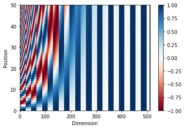
因为该模型并不包括任何的循环(recurrence)或卷积,所以模型添加了位置编码,为模型提供一些关于单词在句子中相对位置的信息。
位置编码向量被加到嵌入(embedding)向量中。嵌入表示一个 d 维空间的标记,在 d 维空间中有着相似含义的标记会离彼此更近。但是,嵌入并没有对在一句话中的词的相对位置进行编码。因此,当加上位置编码后,词将基于它们含义的相似度以及它们在句子中的位置,在 d 维空间中离彼此更近。
参看 位置编码 的 notebook 了解更多信息。计算位置编码的公式如下:
def get_angles(pos, i, d_model):
    angle_rates = 1 / np.power(10000, (2 * (i//2)) / np.float32(d_model))
    return pos * angle_rates
def positional_encoding(position, d_model):
    angle_rads = get_angles(np.arange(position)[:, np.newaxis],
                          np.arange(d_model)[np.newaxis, :],
                          d_model)

    # 将 sin 应用于数组中的偶数索引(indices);2i
    angle_rads[:, 0::2] = np.sin(angle_rads[:, 0::2])

    # 将 cos 应用于数组中的奇数索引;2i+1
    angle_rads[:, 1::2] = np.cos(angle_rads[:, 1::2])

    pos_encoding = angle_rads[np.newaxis, ...]

    return tf.cast(pos_encoding, dtype=tf.float32)
pos_encoding = positional_encoding(50, 512)
print (pos_encoding.shape)

plt.pcolormesh(pos_encoding[0], cmap='RdBu')
plt.xlabel('Dimension')
plt.xlim((0, 512))
plt.ylabel('Position')
plt.colorbar()
plt.show()
(1, 50, 512)
遮挡(Masking)
遮挡一批序列中所有的填充标记(pad tokens)。0 不 mask 掉, 0 就不mask.
def create_padding_mask(seq):
    seq = tf.cast(tf.math.equal(seq, 0), tf.float32)

    # 添加额外的维度来将填充加到
    # 注意力对数(logits)。
    return seq[:, tf.newaxis, tf.newaxis, :]  # (batch_size, 1, 1, seq_len)
x = tf.constant([[7, 6, 0, 0, 1], [1, 2, 3, 0, 0], [0, 0, 0, 4, 5]])
create_padding_mask(x)
<tf.Tensor: shape=(3, 1, 1, 5), dtype=float32, numpy=
array([[[[0., 0., 1., 1., 0.]]],


       [[[0., 0., 0., 1., 1.]]],


       [[[1., 1., 1., 0., 0.]]]], dtype=float32)>
前瞻遮挡(look-ahead mask)用于遮挡一个序列中的后续标记(future tokens)。换句话说,该 mask 表明了不应该使用的条目。
这意味着要预测第三个词,将仅使用第一个和第二个词。与此类似,预测第四个词,仅使用第一个,第二个和第三个词,依此类推。
def create_look_ahead_mask(size):
    mask = 1 - tf.linalg.band_part(tf.ones((size, size)), -1, 0)
    return mask  # (seq_len, seq_len)
x = tf.random.uniform((1, 3))
temp = create_look_ahead_mask(x.shape[1])
temp
<tf.Tensor: shape=(3, 3), dtype=float32, numpy=
array([[0., 1., 1.],
       [0., 0., 1.],
       [0., 0., 0.]], dtype=float32)>
按比缩放的点积注意力(Scaled dot product attention)
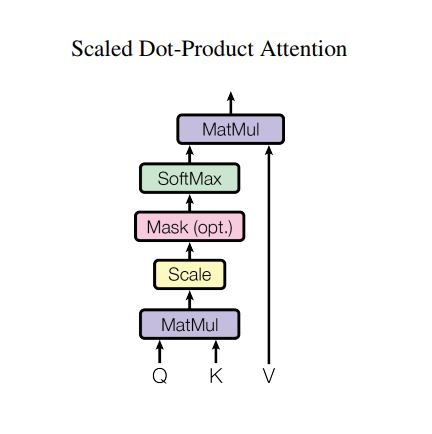
Transformer 使用的注意力函数有三个输入:Q(请求(query))、K(主键(key))、V(数值(value))。用于计算注意力权重的等式为:
点积注意力被缩小了深度的平方根倍。这样做是因为对于较大的深度值,点积的大小会增大,从而推动 softmax 函数往仅有很小的梯度的方向靠拢,导致了一种很硬的(hard)softmax。
例如,假设 Q 和 K 的均值为0,方差为1。它们的矩阵乘积将有均值为0,方差为 dk。因此,dk 的平方根被用于缩放(而非其他数值),因为,Q 和 K 的矩阵乘积的均值本应该为 0,方差本应该为1,这样会获得一个更平缓的 softmax。
遮挡(mask)与 -1e9(接近于负无穷)相乘。这样做是因为遮挡与缩放的 Q 和 K 的矩阵乘积相加,并在 softmax 之前立即应用。目标是将这些单元归零,因为 softmax 的较大负数输入在输出中接近于零。
def scaled_dot_product_attention(q, k, v, mask):
    """计算注意力权重。
    q, k, v 必须具有匹配的前置维度。
    k, v 必须有匹配的倒数第二个维度,例如:seq_len_k = seq_len_v。
    虽然 mask 根据其类型(填充或前瞻)有不同的形状,
    但是 mask 必须能进行广播转换以便求和。

    参数:
    q: 请求的形状 == (..., seq_len_q, depth)
    k: 主键的形状 == (..., seq_len_k, depth)
    v: 数值的形状 == (..., seq_len_v, depth_v)
    mask: Float 张量,其形状能转换成
          (..., seq_len_q, seq_len_k)。默认为None。

    返回值:
    输出,注意力权重
    """

    matmul_qk = tf.matmul(q, k, transpose_b=True)  # (..., seq_len_q, seq_len_k)

    # 缩放 matmul_qk
    dk = tf.cast(tf.shape(k)[-1], tf.float32)
    scaled_attention_logits = matmul_qk / tf.math.sqrt(dk)

    # 将 mask 加入到缩放的张量上。
    if mask is not None:
        scaled_attention_logits += (mask * -1e9)

    # softmax 在最后一个轴(seq_len_k)上归一化,因此分数
    # 相加等于1。
    attention_weights = tf.nn.softmax(scaled_attention_logits, axis=-1)  # (..., seq_len_q, seq_len_k)

    output = tf.matmul(attention_weights, v)  # (..., seq_len_q, depth_v)

    return output, attention_weights
当 softmax 在 K 上进行归一化后,它的值决定了分配到 Q 的重要程度。
输出表示注意力权重和 V(数值)向量的乘积。这确保了要关注的词保持原样,而无关的词将被清除掉。
def print_out(q, k, v):
    temp_out, temp_attn = scaled_dot_product_attention(
      q, k, v, None)
    print ('Attention weights are:')
    print (temp_attn)
    print ('Output is:')
    print (temp_out)
np.set_printoptions(suppress=True)

temp_k = tf.constant([[10,0,0],
                      [0,10,0],
                      [0,0,10],
                      [0,0,10]], dtype=tf.float32)  # (4, 3)

temp_v = tf.constant([[   1,0],
                      [  10,0],
                      [ 100,5],
                      [1000,6]], dtype=tf.float32)  # (4, 2)

# 这条 `请求(query)符合第二个`主键(key)`,
# 因此返回了第二个`数值(value)`。
temp_q = tf.constant([[0, 10, 0]], dtype=tf.float32)  # (1, 3)
print_out(temp_q, temp_k, temp_v)
Attention weights are:
tf.Tensor([[0. 1. 0. 0.]], shape=(1, 4), dtype=float32)
Output is:
tf.Tensor([[10.  0.]], shape=(1, 2), dtype=float32)
# 这条请求符合重复出现的主键(第三第四个),
# 因此,对所有的相关数值取了平均。
temp_q = tf.constant([[0, 0, 10]], dtype=tf.float32)  # (1, 3)
print_out(temp_q, temp_k, temp_v)
Attention weights are:
tf.Tensor([[0.  0.  0.5 0.5]], shape=(1, 4), dtype=float32)
Output is:
tf.Tensor([[550.    5.5]], shape=(1, 2), dtype=float32)
# 这条请求符合第一和第二条主键,
# 因此,对它们的数值去了平均。
temp_q = tf.constant([[10, 10, 0]], dtype=tf.float32)  # (1, 3)
print_out(temp_q, temp_k, temp_v)
Attention weights are:
tf.Tensor([[0.5 0.5 0.  0. ]], shape=(1, 4), dtype=float32)
Output is:
tf.Tensor([[5.5 0. ]], shape=(1, 2), dtype=float32)
将所有请求一起传递。(batch 计算)
temp_q = tf.constant([[0, 0, 10], [0, 10, 0], [10, 10, 0]], dtype=tf.float32)  # (3, 3)
print_out(temp_q, temp_k, temp_v)
Attention weights are:
tf.Tensor(
[[0.  0.  0.5 0.5]
 [0.  1.  0.  0. ]
 [0.5 0.5 0.  0. ]], shape=(3, 4), dtype=float32)
Output is:
tf.Tensor(
[[550.    5.5]
 [ 10.    0. ]
 [  5.5   0. ]], shape=(3, 2), dtype=float32)
多头注意力(Multi-head attention)
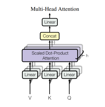
多头注意力由四部分组成:
- 线性层并分拆成多头。
- 按比缩放的点积注意力。
- 多头及联。
- 最后一层线性层。
每个多头注意力块有三个输入:Q(请求)、K(主键)、V(数值)。这些输入经过线性(Dense)层,并分拆成多头。
将上面定义的 scaled_dot_product_attention 函数应用于每个头(进行了广播(broadcasted)以提高效率)。注意力这步必须使用一个恰当的 mask。然后将每个头的注意力输出连接起来(用tf.transpose 和 tf.reshape),并放入最后的 Dense 层。
Q、K、和 V 被拆分到了多个头,而非单个的注意力头,因为多头允许模型共同注意来自不同表示空间的不同位置的信息。在分拆后,每个头部的维度减少,因此总的计算成本与有着全部维度的单个注意力头相同。
class MultiHeadAttention(tf.keras.layers.Layer):
    """
    1 线性层并分拆成多头。
    2 按比缩放的点积注意力。
    3 多头及联。
    4 最后一层线性层。
    """
    def __init__(self, d_model, num_heads):
        super(MultiHeadAttention, self).__init__()
        self.num_heads = num_heads
        self.d_model = d_model

        assert d_model % self.num_heads == 0

        self.depth = d_model // self.num_heads

        self.wq = tf.keras.layers.Dense(d_model)
        self.wk = tf.keras.layers.Dense(d_model)
        self.wv = tf.keras.layers.Dense(d_model)

        self.dense = tf.keras.layers.Dense(d_model)

    def split_heads(self, x, batch_size):
        """分拆最后一个维度到 (num_heads, dimension).
        转置结果使得形状为 (batch_size, num_heads, seq_len, depth)
        """
        x = tf.reshape(x, (batch_size, -1, self.num_heads, self.depth))
        return tf.transpose(x, perm=[0, 2, 1, 3])

    def call(self, v, k, q, mask):
        batch_size = tf.shape(q)[0]

        q = self.wq(q)  # (batch_size, seq_len, d_model)
        k = self.wk(k)  # (batch_size, seq_len, d_model)
        v = self.wv(v)  # (batch_size, seq_len, d_model)

        q = self.split_heads(q, batch_size)  # (batch_size, num_heads, seq_len_q, depth)
        k = self.split_heads(k, batch_size)  # (batch_size, num_heads, seq_len_k, depth)
        v = self.split_heads(v, batch_size)  # (batch_size, num_heads, seq_len_v, depth)

        # scaled_attention.shape == (batch_size, num_heads, seq_len_q, depth)
        # attention_weights.shape == (batch_size, num_heads, seq_len_q, seq_len_k)
        scaled_attention, attention_weights = scaled_dot_product_attention(
            q, k, v, mask)

        scaled_attention = tf.transpose(scaled_attention, perm=[0, 2, 1, 3])  # (batch_size, seq_len_q, num_heads, depth)

        concat_attention = tf.reshape(scaled_attention,
                                      (batch_size, -1, self.d_model))  # (batch_size, seq_len_q, d_model)

        output = self.dense(concat_attention)  # (batch_size, seq_len_q, d_model)

        return output, attention_weights
创建一个 MultiHeadAttention 层进行尝试。在序列中的每个位置 y,MultiHeadAttention 在序列中的所有其他位置运行所有8个注意力头,在每个位置y,返回一个新的同样长度的向量。
temp_mha = MultiHeadAttention(d_model=512, num_heads=8)
y = tf.random.uniform((1, 60, 512))  # (batch_size, encoder_sequence, d_model)
out, attn = temp_mha(y, k=y, q=y, mask=None)
out.shape, attn.shape
(TensorShape([1, 60, 512]), TensorShape([1, 8, 60, 60]))
点式前馈网络(Point wise feed forward network)
点式前馈网络由两层全联接层组成,两层之间有一个 ReLU 激活函数。
def point_wise_feed_forward_network(d_model, dff):
    return tf.keras.Sequential([
      tf.keras.layers.Dense(dff, activation='relu'),  # (batch_size, seq_len, dff)
      tf.keras.layers.Dense(d_model)  # (batch_size, seq_len, d_model)
    ])
sample_ffn = point_wise_feed_forward_network(512, 2048)
sample_ffn(tf.random.uniform((64, 50, 512))).shape
TensorShape([64, 50, 512])
编码与解码(Encoder and decoder)

Transformer 模型与标准的具有注意力机制的序列到序列模型(sequence to sequence with attention model),遵循相同的一般模式。
- 输入语句经过
N个编码器层,为序列中的每个词/标记生成一个输出。 - 解码器关注编码器的输出以及它自身的输入(自注意力)来预测下一个词。
编码器层(Encoder layer)
每个编码器层包括以下子层:
- 多头注意力(有填充遮挡)
- 点式前馈网络(Point wise feed forward networks)。
每个子层在其周围有一个残差连接,然后进行层归一化。残差连接有助于避免深度网络中的梯度消失问题。
每个子层的输出是 LayerNorm(x + Sublayer(x))。归一化是在 d_model(最后一个)维度完成的。Transformer 中有 N 个编码器层。
class EncoderLayer(tf.keras.layers.Layer):
    def __init__(self, d_model, num_heads, dff, rate=0.1):
        super(EncoderLayer, self).__init__()

        self.mha = MultiHeadAttention(d_model, num_heads)
        self.ffn = point_wise_feed_forward_network(d_model, dff)

        self.layernorm1 = tf.keras.layers.LayerNormalization(epsilon=1e-6)
        self.layernorm2 = tf.keras.layers.LayerNormalization(epsilon=1e-6)

        self.dropout1 = tf.keras.layers.Dropout(rate)
        self.dropout2 = tf.keras.layers.Dropout(rate)

    def call(self, x, training, mask):

        attn_output, _ = self.mha(x, x, x, mask)  # (batch_size, input_seq_len, d_model)
        attn_output = self.dropout1(attn_output, training=training)
        # 残差
        out1 = self.layernorm1(x + attn_output)  # (batch_size, input_seq_len, d_model)

        ffn_output = self.ffn(out1)  # (batch_size, input_seq_len, d_model)
        ffn_output = self.dropout2(ffn_output, training=training)
        # 残差
        out2 = self.layernorm2(out1 + ffn_output)  # (batch_size, input_seq_len, d_model)

        return out2
sample_encoder_layer = EncoderLayer(512, 8, 2048)

sample_encoder_layer_output = sample_encoder_layer(
    tf.random.uniform((64, 43, 512)), False, None)

sample_encoder_layer_output.shape  # (batch_size, input_seq_len, d_model)
TensorShape([64, 43, 512])
解码器层(Decoder layer)
每个解码器层包括以下子层:
- 遮挡的多头注意力(前瞻遮挡和填充遮挡)
- 多头注意力(用填充遮挡)。V(数值)和 K(主键)接收编码器输出作为输入。Q(请求)接收遮挡的多头注意力子层的输出。
- 点式前馈网络
每个子层在其周围有一个残差连接,然后进行层归一化。每个子层的输出是 LayerNorm(x + Sublayer(x))。归一化是在 d_model(最后一个)维度完成的。
Transformer 中共有 N 个解码器层。
当 Q 接收到解码器的第一个注意力块的输出,并且 K 接收到编码器的输出时,注意力权重表示根据编码器的输出赋予解码器输入的重要性。换一种说法,解码器通过查看编码器输出和对其自身输出的自注意力,预测下一个词。参看按比缩放的点积注意力部分的演示。
class DecoderLayer(tf.keras.layers.Layer):
    def __init__(self, d_model, num_heads, dff, rate=0.1):
        super(DecoderLayer, self).__init__()

        self.mha1 = MultiHeadAttention(d_model, num_heads)
        self.mha2 = MultiHeadAttention(d_model, num_heads)

        self.ffn = point_wise_feed_forward_network(d_model, dff)

        self.layernorm1 = tf.keras.layers.LayerNormalization(epsilon=1e-6)
        self.layernorm2 = tf.keras.layers.LayerNormalization(epsilon=1e-6)
        self.layernorm3 = tf.keras.layers.LayerNormalization(epsilon=1e-6)

        self.dropout1 = tf.keras.layers.Dropout(rate)
        self.dropout2 = tf.keras.layers.Dropout(rate)
        self.dropout3 = tf.keras.layers.Dropout(rate)


    def call(self, x, enc_output, training,
           look_ahead_mask, padding_mask):
        # enc_output.shape == (batch_size, input_seq_len, d_model)

        attn1, attn_weights_block1 = self.mha1(x, x, x, look_ahead_mask)  # (batch_size, target_seq_len, d_model)
        attn1 = self.dropout1(attn1, training=training)
        out1 = self.layernorm1(attn1 + x)

        # 编码器和解码器之间的attention
        attn2, attn_weights_block2 = self.mha2(
            enc_output, enc_output, out1, padding_mask)  # (batch_size, target_seq_len, d_model)
        attn2 = self.dropout2(attn2, training=training)
        out2 = self.layernorm2(attn2 + out1)  # (batch_size, target_seq_len, d_model)

        ffn_output = self.ffn(out2)  # (batch_size, target_seq_len, d_model)
        ffn_output = self.dropout3(ffn_output, training=training)
        out3 = self.layernorm3(ffn_output + out2)  # (batch_size, target_seq_len, d_model)

        return out3, attn_weights_block1, attn_weights_block2
sample_decoder_layer = DecoderLayer(512, 8, 2048)

sample_decoder_layer_output, _, _ = sample_decoder_layer(
    tf.random.uniform((64, 50, 512)), sample_encoder_layer_output,
    False, None, None)

sample_decoder_layer_output.shape  # (batch_size, target_seq_len, d_model)
TensorShape([64, 50, 512])
编码器(Encoder)
编码器 包括:
- 输入嵌入(Input Embedding)
- 位置编码(Positional Encoding)
- N 个编码器层(encoder layers)
输入经过嵌入(embedding)后,该嵌入与位置编码相加。该加法结果的输出是编码器层的输入。编码器的输出是解码器的输入。
class Encoder(tf.keras.layers.Layer):
    def __init__(self, num_layers, d_model, num_heads, dff, input_vocab_size,
               maximum_position_encoding, rate=0.1):
        super(Encoder, self).__init__()

        self.d_model = d_model
        self.num_layers = num_layers

        self.embedding = tf.keras.layers.Embedding(input_vocab_size, d_model)
        self.pos_encoding = positional_encoding(maximum_position_encoding,
                                                self.d_model)


        self.enc_layers = [EncoderLayer(d_model, num_heads, dff, rate)
                           for _ in range(num_layers)]

        self.dropout = tf.keras.layers.Dropout(rate)

    def call(self, x, training, mask):

        seq_len = tf.shape(x)[1]

        # 将嵌入和位置编码相加。
        x = self.embedding(x)  # (batch_size, input_seq_len, d_model)
        # The reason we increase the embedding values before the addition
        # is to make the positional encoding relatively smaller.
        # This means the original meaning in the embedding vector won’t be lost when we add them together.
        x *= tf.math.sqrt(tf.cast(self.d_model, tf.float32))
        x += self.pos_encoding[:, :seq_len, :]

        x = self.dropout(x, training=training)

        for i in range(self.num_layers):
            x = self.enc_layers[i](x, training, mask)

        return x  # (batch_size, input_seq_len, d_model)
sample_encoder = Encoder(num_layers=2, d_model=512, num_heads=8,
                         dff=2048, input_vocab_size=8500,
                         maximum_position_encoding=10000)

sample_encoder_output = sample_encoder(tf.random.uniform((64, 62)),
                                       training=False, mask=None)

print (sample_encoder_output.shape)  # (batch_size, input_seq_len, d_model)
(64, 62, 512)
解码器(Decoder)
解码器包括:
- 输出嵌入(Output Embedding)
- 位置编码(Positional Encoding)
- N 个解码器层(decoder layers)
目标(target)经过一个嵌入后,该嵌入和位置编码相加。该加法结果是解码器层的输入。解码器的输出是最后的线性层的输入。
class Decoder(tf.keras.layers.Layer):
    def __init__(self, num_layers, d_model, num_heads, dff, target_vocab_size,
               maximum_position_encoding, rate=0.1):
        super(Decoder, self).__init__()

        self.d_model = d_model
        self.num_layers = num_layers

        self.embedding = tf.keras.layers.Embedding(target_vocab_size, d_model)
        self.pos_encoding = positional_encoding(maximum_position_encoding, d_model)

        self.dec_layers = [DecoderLayer(d_model, num_heads, dff, rate)
                           for _ in range(num_layers)]
        self.dropout = tf.keras.layers.Dropout(rate)

    def call(self, x, enc_output, training,
           look_ahead_mask, padding_mask):

        seq_len = tf.shape(x)[1]
        attention_weights = {}

        x = self.embedding(x)  # (batch_size, target_seq_len, d_model)
        x *= tf.math.sqrt(tf.cast(self.d_model, tf.float32))
        x += self.pos_encoding[:, :seq_len, :]

        x = self.dropout(x, training=training)

        for i in range(self.num_layers):
            x, block1, block2 = self.dec_layers[i](x, enc_output, training,
                                                 look_ahead_mask, padding_mask)

            attention_weights['decoder_layer{}_block1'.format(i+1)] = block1
            attention_weights['decoder_layer{}_block2'.format(i+1)] = block2

        # x.shape == (batch_size, target_seq_len, d_model)
        return x, attention_weights
sample_decoder = Decoder(num_layers=2, d_model=512, num_heads=8,
                         dff=2048, target_vocab_size=8000,
                         maximum_position_encoding=5000)

output, attn = sample_decoder(tf.random.uniform((64, 26)),
                              enc_output=sample_encoder_output,
                              training=False, look_ahead_mask=None,
                              padding_mask=None)

output.shape, attn['decoder_layer2_block2'].shape
(TensorShape([64, 26, 512]), TensorShape([64, 8, 26, 62]))
创建 Transformer
Transformer 包括编码器,解码器和最后的线性层。解码器的输出是线性层的输入,返回线性层的输出。
class Transformer(tf.keras.Model):
    def __init__(self, num_layers, d_model, num_heads, dff, input_vocab_size,
               target_vocab_size, pe_input, pe_target, rate=0.1):
        super(Transformer, self).__init__()

        self.encoder = Encoder(num_layers, d_model, num_heads, dff,
                               input_vocab_size, pe_input, rate)

        self.decoder = Decoder(num_layers, d_model, num_heads, dff,
                               target_vocab_size, pe_target, rate)

        self.final_layer = tf.keras.layers.Dense(target_vocab_size)

    def call(self, inp, tar, training, enc_padding_mask,
           look_ahead_mask, dec_padding_mask):

        enc_output = self.encoder(inp, training, enc_padding_mask)  # (batch_size, inp_seq_len, d_model)

        # dec_output.shape == (batch_size, tar_seq_len, d_model)
        dec_output, attention_weights = self.decoder(
            tar, enc_output, training, look_ahead_mask, dec_padding_mask)

        final_output = self.final_layer(dec_output)  # (batch_size, tar_seq_len, target_vocab_size)

        return final_output, attention_weights
sample_transformer = Transformer(
    num_layers=2, d_model=512, num_heads=8, dff=2048,
    input_vocab_size=8500, target_vocab_size=8000,
    pe_input=10000, pe_target=6000)

temp_input = tf.random.uniform((64, 62))
temp_target = tf.random.uniform((64, 26))

fn_out, _ = sample_transformer(temp_input, temp_target, training=False,
                               enc_padding_mask=None,
                               look_ahead_mask=None,
                               dec_padding_mask=None)

fn_out.shape  # (batch_size, tar_seq_len, target_vocab_size)
TensorShape([64, 26, 8000])
配置超参数(hyperparameters)
为了让本示例小且相对较快,已经减小了num_layers、 d_model 和 dff 的值。
Transformer 的基础模型使用的数值为:num_layers=6,d_model = 512,dff = 2048。关于所有其他版本的 Transformer,请查阅论文。
Note:通过改变以下数值,您可以获得在许多任务上达到最先进水平的模型。
num_layers = 4
d_model = 128
dff = 512
num_heads = 8

input_vocab_size = tokenizer_pt.vocab_size + 2
target_vocab_size = tokenizer_en.vocab_size + 2
dropout_rate = 0.1
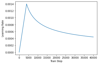
优化器(Optimizer)
根据论文中的公式,将 Adam 优化器与自定义的学习速率调度程序(scheduler)配合使用。
class CustomSchedule(tf.keras.optimizers.schedules.LearningRateSchedule):
    def __init__(self, d_model, warmup_steps=4000):
        super(CustomSchedule, self).__init__()

        self.d_model = d_model
        self.d_model = tf.cast(self.d_model, tf.float32)

        self.warmup_steps = warmup_steps

    def __call__(self, step):
        arg1 = tf.math.rsqrt(step)
        arg2 = step * (self.warmup_steps ** -1.5)

        return tf.math.rsqrt(self.d_model) * tf.math.minimum(arg1, arg2)
learning_rate = CustomSchedule(d_model)

optimizer = tf.keras.optimizers.Adam(learning_rate, beta_1=0.9, beta_2=0.98,
                                     epsilon=1e-9)
temp_learning_rate_schedule = CustomSchedule(d_model)

plt.plot(temp_learning_rate_schedule(tf.range(40000, dtype=tf.float32)))
plt.ylabel("Learning Rate")
plt.xlabel("Train Step")
Text(0.5, 0, 'Train Step')
损失函数与指标(Loss and metrics)
由于目标序列是填充(padded)过的,因此在计算损失函数时,应用填充遮挡非常重要。
loss_object = tf.keras.losses.SparseCategoricalCrossentropy(
    from_logits=True, reduction='none')
mask in mask = tf.math.logical_not(tf.math.equal(real, 0)) is taking care of the PADDING.
So, in your batch you would have sentences of different length and you do 0 padding to make all of them of equal length
(think about I have an apple v/s It's a good day to play football in the sun)
But, it doesn't make sense to include the 0 padded section in the loss calculation - hence, it's first looking into indices where you have a 0 and using multiplication later on to make their loss contribution 0.
def loss_function(real, pred):
    mask = tf.math.logical_not(tf.math.equal(real, 0))
    loss_ = loss_object(real, pred)

    mask = tf.cast(mask, dtype=loss_.dtype)
    loss_ *= mask

    return tf.reduce_mean(loss_)
train_loss = tf.keras.metrics.Mean(name='train_loss')
train_accuracy = tf.keras.metrics.SparseCategoricalAccuracy(
    name='train_accuracy')
训练与检查点(Training and checkpointing)
transformer = Transformer(num_layers, d_model, num_heads, dff,
                          input_vocab_size, target_vocab_size,
                          pe_input=input_vocab_size,
                          pe_target=target_vocab_size,
                          rate=dropout_rate)
def create_masks(inp, tar):
    # 编码器填充遮挡
    enc_padding_mask = create_padding_mask(inp)

    # 在解码器的第二个注意力模块使用。
    # 该填充遮挡用于遮挡编码器的输出。
    dec_padding_mask = create_padding_mask(inp)

    # 在解码器的第一个注意力模块使用。
    # 用于填充(pad)和遮挡(mask)解码器获取到的输入的后续标记(future tokens)。
    look_ahead_mask = create_look_ahead_mask(tf.shape(tar)[1])
    dec_target_padding_mask = create_padding_mask(tar)
    # 把该掩盖的都给掩盖掉
    combined_mask = tf.maximum(dec_target_padding_mask, look_ahead_mask)

    return enc_padding_mask, combined_mask, dec_padding_mask
创建检查点的路径和检查点管理器(manager)。这将用于在每 n 个周期(epochs)保存检查点。
checkpoint_path = "./checkpoints/train"

ckpt = tf.train.Checkpoint(transformer=transformer,
                           optimizer=optimizer)

ckpt_manager = tf.train.CheckpointManager(ckpt, checkpoint_path, max_to_keep=5)

# 如果检查点存在,则恢复最新的检查点。
if ckpt_manager.latest_checkpoint:
    ckpt.restore(ckpt_manager.latest_checkpoint)
    print ('Latest checkpoint restored!!')
目标(target)被分成了 tar_inp 和 tar_real。tar_inp 作为输入传递到解码器。tar_real 是位移了 1 的同一个输入:在 tar_inp 中的每个位置,tar_real 包含了应该被预测到的下一个标记(token)。
例如,sentence = "SOS A lion in the jungle is sleeping EOS"
tar_inp = "SOS A lion in the jungle is sleeping"
tar_real = "A lion in the jungle is sleeping EOS"
Transformer 是一个自回归(auto-regressive)模型:它一次作一个部分的预测,然后使用到目前为止的自身的输出来决定下一步要做什么。
在训练过程中,本示例使用了 teacher-forcing 的方法(就像文本生成教程中一样)。无论模型在当前时间步骤下预测出什么,teacher-forcing 方法都会将真实的输出传递到下一个时间步骤上。
当 transformer 预测每个词时,自注意力(self-attention)功能使它能够查看输入序列中前面的单词,从而更好地预测下一个单词。
为了防止模型在期望的输出上达到峰值,模型使用了前瞻遮挡(look-ahead mask)。
EPOCHS = 20
# 该 @tf.function 将追踪-编译 train_step 到 TF 图中,以便更快地
# 执行。该函数专用于参数张量的精确形状。为了避免由于可变序列长度或可变
# 批次大小(最后一批次较小)导致的再追踪,使用 input_signature 指定
# 更多的通用形状。

train_step_signature = [
    tf.TensorSpec(shape=(None, None), dtype=tf.int64),
    tf.TensorSpec(shape=(None, None), dtype=tf.int64),
]

@tf.function(input_signature=train_step_signature)
def train_step(inp, tar):
  tar_inp = tar[:, :-1]
  tar_real = tar[:, 1:]

  enc_padding_mask, combined_mask, dec_padding_mask = create_masks(inp, tar_inp)

  with tf.GradientTape() as tape:
    predictions, _ = transformer(inp, tar_inp,
                                 True,
                                 enc_padding_mask,
                                 combined_mask,
                                 dec_padding_mask)
    loss = loss_function(tar_real, predictions)

  gradients = tape.gradient(loss, transformer.trainable_variables)
  optimizer.apply_gradients(zip(gradients, transformer.trainable_variables))

  train_loss(loss)
  train_accuracy(tar_real, predictions)
葡萄牙语作为输入语言,英语为目标语言。
for epoch in range(EPOCHS):
    start = time.time()

    train_loss.reset_states()
    train_accuracy.reset_states()

    # inp -> portuguese, tar -> english
    for (batch, (inp, tar)) in enumerate(train_dataset):
        train_step(inp, tar)

        if batch % 50 == 0:
            print ('Epoch {} Batch {} Loss {:.4f} Accuracy {:.4f}'.format(
                  epoch + 1, batch, train_loss.result(), train_accuracy.result()))

    if (epoch + 1) % 5 == 0:
        ckpt_save_path = ckpt_manager.save()
        print ('Saving checkpoint for epoch {} at {}'.format(epoch+1,
                                                             ckpt_save_path))

    print ('Epoch {} Loss {:.4f} Accuracy {:.4f}'.format(epoch + 1,
                                                train_loss.result(),
                                                train_accuracy.result()))

    print ('Time taken for 1 epoch: {} secs\n'.format(time.time() - start))
评估(Evaluate)
以下步骤用于评估:
- 用葡萄牙语分词器(
tokenizer_pt)编码输入语句。此外,添加开始和结束标记,这样输入就与模型训练的内容相同。这是编码器输入。 - 解码器输入为
start token == tokenizer_en.vocab_size。 - 计算填充遮挡和前瞻遮挡。
解码器通过查看编码器输出和它自身的输出(自注意力)给出预测。- 选择最后一个词并计算它的 argmax。
- 将预测的词连接到解码器输入,然后传递给解码器。
- 在这种方法中,解码器根据它预测的之前的词预测下一个。
Note:这里使用的模型具有较小的能力以保持相对较快,因此预测可能不太正确。要复现论文中的结果,请使用全部数据集,并通过修改上述超参数来使用基础 transformer 模型或者 transformer XL。
def evaluate(inp_sentence):
    start_token = [tokenizer_pt.vocab_size]
    end_token = [tokenizer_pt.vocab_size + 1]

    # 输入语句是葡萄牙语,增加开始和结束标记
    inp_sentence = start_token + tokenizer_pt.encode(inp_sentence) + end_token
    encoder_input = tf.expand_dims(inp_sentence, 0)

    # 因为目标是英语,输入 transformer 的第一个词应该是
    # 英语的开始标记。
    decoder_input = [tokenizer_en.vocab_size]
    output = tf.expand_dims(decoder_input, 0)

    for i in range(MAX_LENGTH):
        enc_padding_mask, combined_mask, dec_padding_mask = create_masks(
            encoder_input, output)

        # predictions.shape == (batch_size, seq_len, vocab_size)
        predictions, attention_weights = transformer(encoder_input,
                                                     output,
                                                     False,
                                                     enc_padding_mask,
                                                     combined_mask,
                                                     dec_padding_mask)

        # 从 seq_len 维度选择最后一个词
        predictions = predictions[: ,-1:, :]  # (batch_size, 1, vocab_size)

        predicted_id = tf.cast(tf.argmax(predictions, axis=-1), tf.int32)

        # 如果 predicted_id 等于结束标记,就返回结果
        if predicted_id == tokenizer_en.vocab_size+1:
            return tf.squeeze(output, axis=0), attention_weights

        # 连接 predicted_id 与输出,作为解码器的输入传递到解码器。
        output = tf.concat([output, predicted_id], axis=-1)

    return tf.squeeze(output, axis=0), attention_weights
def plot_attention_weights(attention, sentence, result, layer):
  fig = plt.figure(figsize=(16, 8))

  sentence = tokenizer_pt.encode(sentence)

  attention = tf.squeeze(attention[layer], axis=0)

  for head in range(attention.shape[0]):
    ax = fig.add_subplot(2, 4, head+1)

    # 画出注意力权重
    ax.matshow(attention[head][:-1, :], cmap='viridis')

    fontdict = {'fontsize': 10}

    ax.set_xticks(range(len(sentence)+2))
    ax.set_yticks(range(len(result)))

    ax.set_ylim(len(result)-1.5, -0.5)

    ax.set_xticklabels(
        ['<start>']+[tokenizer_pt.decode([i]) for i in sentence]+['<end>'],
        fontdict=fontdict, rotation=90)

    ax.set_yticklabels([tokenizer_en.decode([i]) for i in result
                        if i < tokenizer_en.vocab_size],
                       fontdict=fontdict)

    ax.set_xlabel('Head {}'.format(head+1))

  plt.tight_layout()
  plt.show()
def translate(sentence, plot=''):
  result, attention_weights = evaluate(sentence)

  predicted_sentence = tokenizer_en.decode([i for i in result
                                            if i < tokenizer_en.vocab_size])

  print('Input: {}'.format(sentence))
  print('Predicted translation: {}'.format(predicted_sentence))

  if plot:
    plot_attention_weights(attention_weights, sentence, result, plot)
translate("este é um problema que temos que resolver.")
print ("Real translation: this is a problem we have to solve .")
Input: este é um problema que temos que resolver.
Predicted translation: this is a problem that we have to solve the united states is that we have to solve the world .
Real translation: this is a problem we have to solve .
translate("os meus vizinhos ouviram sobre esta ideia.")
print ("Real translation: and my neighboring homes heard about this idea .")
Input: os meus vizinhos ouviram sobre esta ideia.
Predicted translation: my neighbors heard about this idea .
Real translation: and my neighboring homes heard about this idea .
translate("vou então muito rapidamente partilhar convosco algumas histórias de algumas coisas mágicas que aconteceram.")
print ("Real translation: so i 'll just share with you some stories very quickly of some magical things that have happened .")
Input: vou então muito rapidamente partilhar convosco algumas histórias de algumas coisas mágicas que aconteceram.
Predicted translation: so i 'm going to share with you a couple of exciting stories of some magical things that happened .
Real translation: so i 'll just share with you some stories very quickly of some magical things that have happened .
您可以为 plot 参数传递不同的层和解码器的注意力模块。
translate("este é o primeiro livro que eu fiz.", plot='decoder_layer4_block2')
print ("Real translation: this is the first book i've ever done.")
Input: este é o primeiro livro que eu fiz.
Predicted translation: this is the first book that i made .
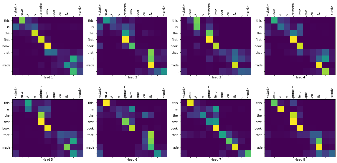
Real translation: this is the first book i've ever done.
总结
在本教程中,您已经学习了位置编码,多头注意力,遮挡的重要性以及如何创建一个 transformer。
尝试使用一个不同的数据集来训练 transformer。您可也可以通过修改上述的超参数来创建基础 transformer 或者 transformer XL。您也可以使用这里定义的层来创建 BERT 并训练最先进的模型。此外,您可以实现 beam search 得到更好的预测。